A two-moderator model, with the moderators affecting the effects of different predictors.
Format
A data frame with 200 rows and 6 variables:
- y
Outcome variable. Numeric.
- x1
Predictor 1. Numeric.
- x2
Predictor 2. Numeric.
- w1
Moderator 1. Numeric.
- w2
Moderator 2. Numeric.
- c1
Control variable. Numeric.
- c2
Control variable. Numeric.
Examples
library(lavaan)
data(data_mod_2x2w)
lm_out <- lm(y ~ x1*w1 + x2*w2 + c1 + c2, data_mod_2x2w)
out1 <- cond_effects(
wlevels = "w1",
x = "x1",
fit = lm_out
)
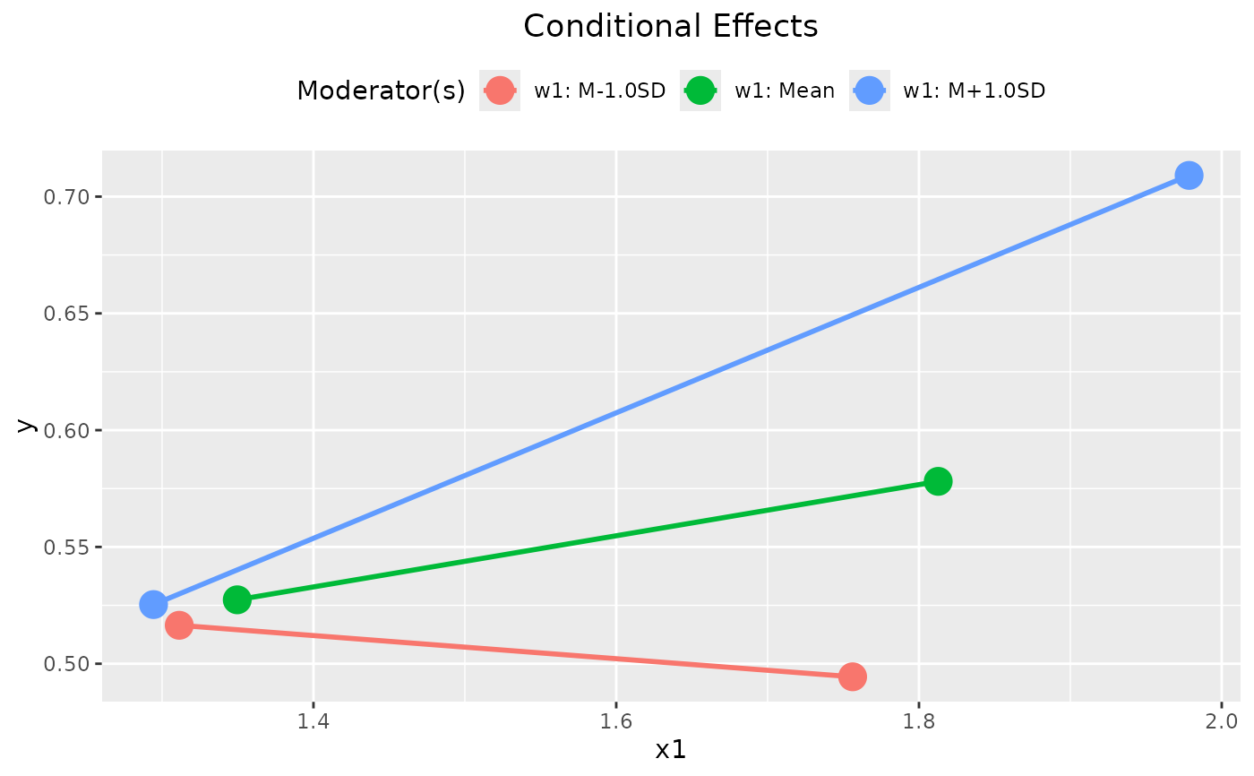
out1
#>
#> == Conditional effects ==
#>
#> Path: x1 -> y
#> Conditional on moderator(s): w1
#> Moderator(s) represented by: w1
#> Computation Formula:
#> (b.y~x1 + (b.x1:w1)*(w1))
#>
#> [w1] (w1) ind SE Stat pvalue Sig CI.lo CI.hi
#> 1 M+1.0SD 2.285 0.269 0.023 11.801 0.000 *** 0.224 0.313
#> 2 Mean 2.032 0.110 0.021 5.222 0.000 *** 0.068 0.151
#> 3 M-1.0SD 1.779 -0.050 0.033 -1.513 0.132 -0.114 0.015
#>
#> - [SE] are regression standard errors.
#> - [Stat] are the t statistics used to test the effects.
#> - [pvalue] are p-values computed from 'Stat'.
#> - [Sig]: 0 ‘***’ 0.001 ‘**’ 0.01 ‘*’ 0.05 ‘ ’ 1.
#> - [CI.lo to CI.hi] are 95.0% confidence interval computed from
#> regression standard errors.
#> - The 'ind' column shows the conditional effects.
#> - Call ‘print_all_cond_indirect_effects()’ to print the detailed
#> outputs of all levels.
#>
plot(out1, graph_type = "tumble")
 out2 <- cond_effects(
wlevels = "w2",
x = "x2",
fit = lm_out
)
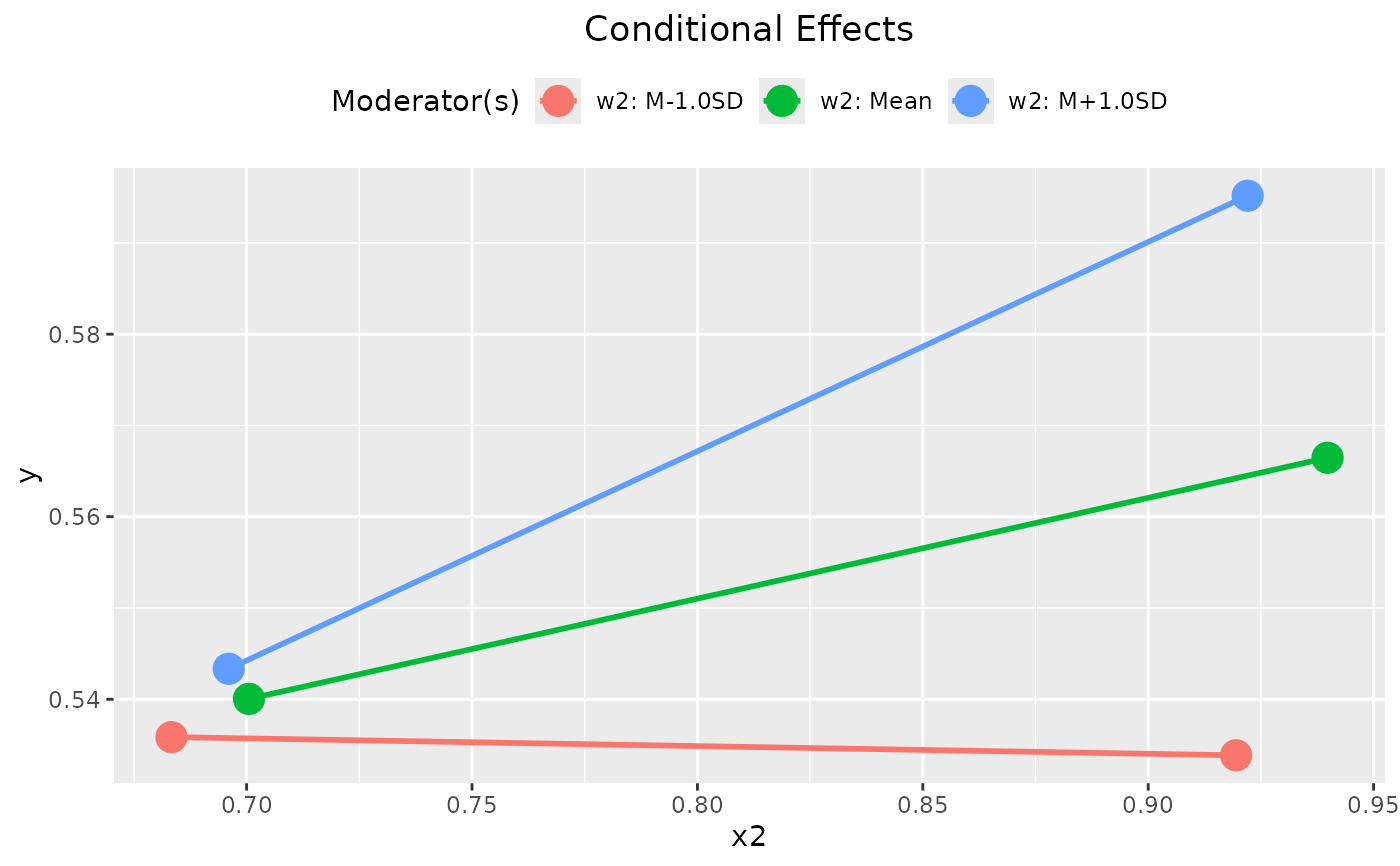
out2
#>
#> == Conditional effects ==
#>
#> Path: x2 -> y
#> Conditional on moderator(s): w2
#> Moderator(s) represented by: w2
#> Computation Formula:
#> (b.y~x2 + (b.x2:w2)*(w2))
#>
#> [w2] (w2) ind SE Stat pvalue Sig CI.lo CI.hi
#> 1 M+1.0SD 1.666 0.229 0.071 3.218 0.002 ** 0.089 0.370
#> 2 Mean 1.332 0.110 0.047 2.358 0.019 * 0.018 0.203
#> 3 M-1.0SD 0.998 -0.008 0.070 -0.120 0.904 -0.147 0.130
#>
#> - [SE] are regression standard errors.
#> - [Stat] are the t statistics used to test the effects.
#> - [pvalue] are p-values computed from 'Stat'.
#> - [Sig]: 0 ‘***’ 0.001 ‘**’ 0.01 ‘*’ 0.05 ‘ ’ 1.
#> - [CI.lo to CI.hi] are 95.0% confidence interval computed from
#> regression standard errors.
#> - The 'ind' column shows the conditional effects.
#> - Call ‘print_all_cond_indirect_effects()’ to print the detailed
#> outputs of all levels.
#>
plot(out2, graph_type = "tumble")
out2 <- cond_effects(
wlevels = "w2",
x = "x2",
fit = lm_out
)
out2
#>
#> == Conditional effects ==
#>
#> Path: x2 -> y
#> Conditional on moderator(s): w2
#> Moderator(s) represented by: w2
#> Computation Formula:
#> (b.y~x2 + (b.x2:w2)*(w2))
#>
#> [w2] (w2) ind SE Stat pvalue Sig CI.lo CI.hi
#> 1 M+1.0SD 1.666 0.229 0.071 3.218 0.002 ** 0.089 0.370
#> 2 Mean 1.332 0.110 0.047 2.358 0.019 * 0.018 0.203
#> 3 M-1.0SD 0.998 -0.008 0.070 -0.120 0.904 -0.147 0.130
#>
#> - [SE] are regression standard errors.
#> - [Stat] are the t statistics used to test the effects.
#> - [pvalue] are p-values computed from 'Stat'.
#> - [Sig]: 0 ‘***’ 0.001 ‘**’ 0.01 ‘*’ 0.05 ‘ ’ 1.
#> - [CI.lo to CI.hi] are 95.0% confidence interval computed from
#> regression standard errors.
#> - The 'ind' column shows the conditional effects.
#> - Call ‘print_all_cond_indirect_effects()’ to print the detailed
#> outputs of all levels.
#>
plot(out2, graph_type = "tumble")