Monte Carlo Confidence Intervals with Multiple Imputation
Shu Fai Cheung & Sing-Hang Cheung
2026-03-26
Source:vignettes/do_mc_lavaan_mi.Rmd
do_mc_lavaan_mi.RmdIntroduction
This article is a brief illustration of how to use
do_mc() from the package manymome (Cheung & Cheung,
2024) for a model fitted to multiple imputation datasets to generate
Monte Carlo estimates, which can be used by
indirect_effect() and cond_indirect_effects()
to form Monte Carlo confidence intervals in the presence of missing
data.
For the details of using do_mc(), please refer to
vignette("do_mc"). This article assumes that readers know
how to use do_mc() and will focus on using it with a model
estimated by multiple imputation.
It only supports a model fitted by lavaan.mi::sem.mi()
or lavaan.mi::lavaan.mi().
How It Works
When used with multiple imputation, do_mc() retrieves
the pooled point estimates and variance-covariance matrix of free model
parameters and then generates a number of sets of simulated sample
estimates using a multivariate normal distribution. Other parameters and
implied variances, covariances, and means of variables are then
generated from these simulated estimates.
When a % Monte Carlo confidence interval is requested, the th percentile and the th percentile are used to form the confidence interval. For a 95% Monte Carlo confidence interval, the 2.5th percentile and 97.5th percentile will be used.
The Workflow
The following workflow will be demonstrated;
Generate datasets using multiple imputation, not covered here (please refer to guides on
miceorAmelia, the two packages supported bylavaan.mi::sem.mi()andlavaan.mi::lavaan.mi()).Fit the model using
lavaan.mi::sem.mi()orlavaan.mi::lavaan.mi().Use
do_mc()to generate the Monte Carlo estimates.Call other functions (e.g,
indirect_effect()andcond_indirect_effects()) to compute the desired effects and form Monte Carlo confidence intervals.
Demonstration
Multiple Imputation
This data set, with missing data introduced, will be used for illustration.
library(manymome)
dat <- data_med
dat[1, 1] <- dat[2, 3] <- dat[3, 5] <- dat[4, 3] <- dat[5, 2] <- NA
head(dat)
#>           x        m        y       c1       c2
#> 1        NA 17.89644 20.73893 1.426513 6.103290
#> 2  8.331493 17.92150       NA 2.940388 3.832698
#> 3 10.327471 17.83178 22.14201 3.012678       NA
#> 4 11.196969 20.01750       NA 3.120056 4.654931
#> 5 11.887811       NA 28.47312 4.440018 3.959033
#> 6  8.198297 16.95198 20.73549 2.495083 3.763712
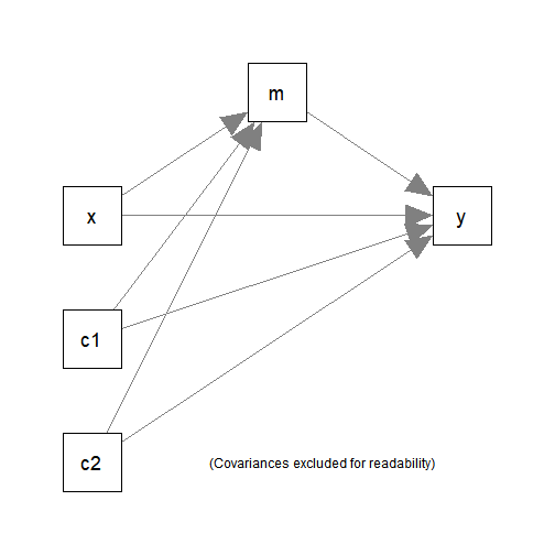
It has one predictor (x), one mediator (m),
one outcome variable (y), and two control variables
(c1 and c2).
The following simple mediation model with two control variables
(c1 and c2) will be fitted:

In practice, the imputation model needs to be decided and checked
(van Buuren, 2018). For the sake of illustration, we just use the
default of mice::mice() to do the imputation:
library(mice)
set.seed(26245)
out_mice <- mice(dat, m = 5, printFlag = FALSE)
dat_mi <- complete(out_mice, action = "all")
# The first imputed dataset
head(dat_mi[[1]])
#>           x        m        y       c1       c2
#> 1  9.762412 17.89644 20.73893 1.426513 6.103290
#> 2  8.331493 17.92150 25.68452 2.940388 3.832698
#> 3 10.327471 17.83178 22.14201 3.012678 3.969419
#> 4 11.196969 20.01750 24.87107 3.120056 4.654931
#> 5 11.887811 20.82502 28.47312 4.440018 3.959033
#> 6  8.198297 16.95198 20.73549 2.495083 3.763712
# The last imputed dataset
head(dat_mi[[5]])
#>           x        m        y       c1       c2
#> 1  8.301276 17.89644 20.73893 1.426513 6.103290
#> 2  8.331493 17.92150 22.93143 2.940388 3.832698
#> 3 10.327471 17.83178 22.14201 3.012678 6.238426
#> 4 11.196969 20.01750 26.90840 3.120056 4.654931
#> 5 11.887811 20.82502 28.47312 4.440018 3.959033
#> 6  8.198297 16.95198 20.73549 2.495083 3.763712
Fit a Model by lavaan.mi::sem.mi()
We then fit the model by lavaan.mi::sem.mi():
library(lavaan.mi)
mod <-
"
m ~ x + c1 + c2
y ~ m + x + c1 + c2
"
fit_lavaan <- sem.mi(model = mod,
                     data = dat_mi)
summary(fit_lavaan)
#> lavaan.mi object fit to 5 imputed data sets using:
#>  - lavaan    (0.6-21)
#>  - lavaan.mi (0.1-0)
#> See class?lavaan.mi help page for available methods.
#>
#> Convergence information:
#> The model converged on 5 imputed data sets.
#> Standard errors were available for all imputations.
#>
#>   Estimator                                         ML
#>   Optimization method                           NLMINB
#>   Number of model parameters                         9
#>
#>   Number of observations                           100
#>
#> Model Test User Model:
#>
#>   Test statistic                                 0.000
#>   Degrees of freedom                                 0
#>   P-value                                        1.000
#>   Pooling method                                    D4
#>
#> Parameter Estimates:
#>
#>   Standard errors                                   Standard
#>   Information                                       Expected
#>   Information saturated (h1) model                Structured
#>
#>   Pooled across imputations             Rubin's (1987) rules
#>   Augment within-imputation variance    Scale by average RIV
#>   Wald test for pooled parameters         t(df) distribution
#>
#>   Pooled t statistics with df >= 1000 are displayed with
#>   df = Inf(inity) to save space. Although the t distribution
#>   with large df closely approximates a standard normal
#>   distribution, exact df for reporting these t tests can be
#>   obtained from parameterEstimates.mi()
#>
#>
#> Regressions:
#>                    Estimate  Std.Err  t-value       df  P(>|t|)
#>   m ~
#>     x                 0.891    0.080   11.117      Inf    0.000
#>     c1                0.162    0.077    2.118      Inf    0.034
#>     c2               -0.114    0.102   -1.117      Inf    0.264
#>   y ~
#>     m                 0.736    0.251    2.935      Inf    0.003
#>     x                 0.616    0.298    2.065  383.680    0.040
#>     c1                0.181    0.193    0.939      Inf    0.348
#>     c2               -0.156    0.254   -0.616      Inf    0.538
#>
#> Variances:
#>                    Estimate  Std.Err  t-value       df  P(>|t|)
#>    .m                 0.682    0.098    6.959      Inf    0.000
#>    .y                 4.151    0.597    6.958      Inf    0.000
Generate Monte Carlo Estimates
The other steps are identical to those illustrated in
vignette("do_mc"). It and related functions will use the
pooled point estimates and variance-covariance matrix when they detect
that the model is fitted by lavaan.mi::sem.mi() or
lavaan.mi::lavaan.mi() (i.e., the fit object is of the
class lavaan.mi).
We call do_mc() on the output of
lavaan.mi::sem.mi() to generate the Monte Carlo estimates
of all free parameters and the implied statistics, such as the
variances of m and y, which are not free
parameters but are needed to form the confidence interval of the
standardized indirect effect.
mc_out_lavaan <- do_mc(fit = fit_lavaan,
                       R = 10000,
                       seed = 4234)
#> Stage 1: Simulate estimates
#> Stage 2: Compute implied statistics
Usually, just three arguments are needed:
fit: The output oflavaan::sem().R: The number of Monte Carlo replications. Should be at least 10000 in real research.seed: The seed for the random number generator. To be used byset.seed(). It is recommended to set this argument such that the results are reproducible.
Parallel processing is not used. However, the time taken is rarely long because there is no need to refit the model many times.
For the structure of the output, please refer to
vignette("do_mc").
Using the Output of do_mc() in Other Functions of
manymome
When calling indirect_effect() or
cond_indirect_effects(), the argument mc_out
can be assigned the output of do_mc(). They will then
retrieve the stored simulated estimates to form the Monte Carlo
confidence intervals, if requested.
out_lavaan <- indirect_effect(x = "x",
                              y = "y",
                              m = "m",
                              fit = fit_lavaan,
                              mc_ci = TRUE,
                              mc_out = mc_out_lavaan)
out_lavaan
#>
#> == Indirect Effect  ==
#>
#>  Path:                 x -> m -> y
#>  Indirect Effect:      0.656
#>  95.0% Monte Carlo CI: [0.213 to 1.124]
#>
#> Computation Formula:
#>   (b.m~x)*(b.y~m)
#>
#> Computation:
#>   (0.89141)*(0.73569)
#>
#>
#> Monte Carlo confidence interval with 10000 replications.
#>
#> Coefficients of Component Paths:
#>  Path Coefficient
#>   m~x       0.891
#>   y~m       0.736
Reusing the simulated estimates can ensure that all analysis with Monte Carlo confidence intervals are based on the same set of simulated estimates.
Limitation
Monte Carlo confidence intervals require the variance-covariance
matrix of all free parameters. Therefore, only models fitted by
lavaan::sem() and (since 0.1.9.8)
lavaan.mi::sem.mi() or lavaan.mi::lavaan.mi()
are supported. Models fitted by stats::lm() do not have a
variance-covariance matrix for the regression coefficients from two or
more regression models and so are not supported by
do_mc().
Further Information
For further information on do_mc(), please refer to its
help page.
Reference
Cheung, S. F., & Cheung, S.-H. (2024). manymome: An R package for computing the indirect effects, conditional effects, and conditional indirect effects, standardized or unstandardized, and their bootstrap confidence intervals, in many (though not all) models. Behavior Research Methods, 56(5), 4862–4882. https://doi.org/10.3758/s13428-023-02224-z
van Buuren, S. (2018). Flexible imputation of missing data (2nd Ed.). CRC Press, Taylor and Francis Group.