Mediation Models with Latent Variables
Shu Fai Cheung & Sing-Hang Cheung
2026-03-26
Source:vignettes/med_lav.Rmd
med_lav.RmdIntroduction
This article is a brief illustration of how
indirect_effect() from the package manymome (Cheung & Cheung,
2024) can be used to estimate the indirect effects among latent
variables and form bootstrap confidence intervals for these effects.
Data Set and Model
This is the sample dataset used for illustration:
library(manymome)
dat <- data_sem
print(round(head(dat), 1))
#>    x01  x02  x03  x04  x05  x06  x07  x08  x09  x10  x11  x12  x13  x14
#> 1  0.2 -1.1 -0.2  2.7 -0.1  2.2  1.7  0.2 -1.9 -2.1 -0.9 -0.5 -0.6 -1.5
#> 2  0.1  0.3  0.9 -0.5 -1.0  0.8 -0.3 -0.9  0.8 -1.5 -0.7  1.0 -0.8 -1.4
#> 3 -0.1 -0.1  2.4 -0.2 -0.1 -1.6 -1.9 -2.4 -0.3 -0.2  0.5 -0.7  0.2 -0.7
#> 4 -0.5  1.1 -0.7 -0.5  1.0 -0.6 -0.9 -1.5 -1.5 -0.5 -2.2 -1.6 -0.8 -0.2
#> 5 -0.8 -0.3 -0.9 -0.2  0.3 -2.1 -0.5 -1.8 -0.1 -2.7 -0.4 -1.2  0.3 -2.6
#> 6  0.9  0.3  0.3  1.0 -1.8 -0.4  0.8 -0.4 -1.1 -2.1  0.4  0.0 -0.3  2.2
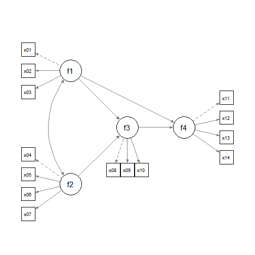
This dataset has 14 variables, which are indicators of four latent
factors: f1, f2, f3, and
f4.
Suppose this is the model to be fitted:

This model can be fitted by lavaan::sem():
mod <-
"
f1 =~ x01 + x02 + x03
f2 =~ x04 + x05 + x06 + x07
f3 =~ x08 + x09 + x10
f4 =~ x11 + x12 + x13 + x14
f3 ~  f1 + f2
f4 ~  f1 + f3
"
fit_med <- sem(model = mod,
               data = dat)
These are the estimates of the paths between the latent variables:
est <- parameterEstimates(fit_med)
est[est$op == "~", ]
#>    lhs op rhs   est    se     z pvalue ci.lower ci.upper
#> 15  f3  ~  f1 0.243 0.120 2.018  0.044    0.007    0.479
#> 16  f3  ~  f2 0.326 0.102 3.186  0.001    0.125    0.526
#> 17  f4  ~  f1 0.447 0.125 3.592  0.000    0.203    0.692
#> 18  f4  ~  f3 0.402 0.090 4.445  0.000    0.225    0.579
Suppose that for the free parameters, we would like to use ML to form the confidence intervals. For indirect effects, we want to use bootstrapping.
Generating Bootstrap Estimates
Although bootstrap estimates can be generated and stored the first
time we call indirect_effect(), we illustrate using
do_boot() to generate the bootstrap estimates to be used by
indirect_effect():
boot_out_med <- do_boot(fit_med,
                        R = 100,
                        seed = 98171,
                        ncores = 1)
Please see vignette("do_boot") or the help page of
do_boot() on how to use this function. In real research,
R, the number of bootstrap samples, should be set to 2000
or even 5000. The argument ncores can usually be omitted
unless users want to manually control the number of CPU cores to be used
in parallel processing.
Indirect Effects
Even though path coefficients are not labelled, we can still use
indirect_effect() to estimate the indirect effect and form
its bootstrap confidence interval for any path in the model. By reusing
the generated bootstrap estimates, there is no need to repeat the
resampling and estimation.
Suppose we want to estimate the indirect effect from f1
to f4 through f3:
out_f1f3f4 <- indirect_effect(x = "f1",
                              y = "f4",
                              m = "f3",
                              fit = fit_med,
                              boot_ci = TRUE,
                              boot_out = boot_out_med)
out_f1f3f4
#>
#> == Indirect Effect  ==
#>
#>  Path:               f1 -> f3 -> f4
#>  Indirect Effect:    0.098
#>  95.0% Bootstrap CI: [-0.007 to 0.216]
#>
#> Computation Formula:
#>   (b.f3~f1)*(b.f4~f3)
#>
#> Computation:
#>   (0.24307)*(0.40186)
#>
#>
#> Percentile confidence interval formed by nonparametric bootstrapping
#> with 100 bootstrap samples.
#>
#> Coefficients of Component Paths:
#>   Path Coefficient
#>  f3~f1       0.243
#>  f4~f3       0.402
The indirect effect is 0.098, with 95% confidence interval [-0.007, 0.216].
Similarly, we can estimate the indirect effect from f2
to f4 through f3:
out_f2f3f4 <- indirect_effect(x = "f2",
                              y = "f4",
                              m = "f3",
                              fit = fit_med,
                              boot_ci = TRUE,
                              boot_out = boot_out_med)
out_f2f3f4
#>
#> == Indirect Effect  ==
#>
#>  Path:               f2 -> f3 -> f4
#>  Indirect Effect:    0.131
#>  95.0% Bootstrap CI: [0.049 to 0.254]
#>
#> Computation Formula:
#>   (b.f3~f2)*(b.f4~f3)
#>
#> Computation:
#>   (0.32561)*(0.40186)
#>
#>
#> Percentile confidence interval formed by nonparametric bootstrapping
#> with 100 bootstrap samples.
#>
#> Coefficients of Component Paths:
#>   Path Coefficient
#>  f3~f2       0.326
#>  f4~f3       0.402
The indirect effect is 0.131, with 95% confidence interval [0.049, 0.254].
Standardized Indirect effects
The standardized indirect effect from f1 to
f4 through f3 can be estimated by setting
standardized_x and standardized_y to
`TRUE:
std_f1f3f4 <- indirect_effect(x = "f1",
                              y = "f4",
                              m = "f3",
                              fit = fit_med,
                              boot_ci = TRUE,
                              boot_out = boot_out_med,
                              standardized_x = TRUE,
                              standardized_y = TRUE)
std_f1f3f4
#>
#> == Indirect Effect (Both 'f1' and 'f4' Standardized) ==
#>
#>  Path:               f1 -> f3 -> f4
#>  Indirect Effect:    0.073
#>  95.0% Bootstrap CI: [-0.005 to 0.157]
#>
#> Computation Formula:
#>   (b.f3~f1)*(b.f4~f3)*sd_f1/sd_f4
#>
#> Computation:
#>   (0.24307)*(0.40186)*(0.87470)/(1.17421)
#>
#>
#> Percentile confidence interval formed by nonparametric bootstrapping
#> with 100 bootstrap samples.
#>
#> Coefficients of Component Paths:
#>   Path Coefficient
#>  f3~f1       0.243
#>  f4~f3       0.402
#>
#> NOTE:
#> - The effects of the component paths are from the model, not
#>   standardized.
The standardized indirect effect is 0.073, with 95% confidence interval [-0.005, 0.157].
Similarly, we can estimate the standardized indirect effect from
f2 to f4 through f3:
std_f2f3f4 <- indirect_effect(x = "f2",
                              y = "f4",
                              m = "f3",
                              fit = fit_med,
                              boot_ci = TRUE,
                              boot_out = boot_out_med,
                              standardized_x = TRUE,
                              standardized_y = TRUE)
std_f2f3f4
#>
#> == Indirect Effect (Both 'f2' and 'f4' Standardized) ==
#>
#>  Path:               f2 -> f3 -> f4
#>  Indirect Effect:    0.116
#>  95.0% Bootstrap CI: [0.044 to 0.204]
#>
#> Computation Formula:
#>   (b.f3~f2)*(b.f4~f3)*sd_f2/sd_f4
#>
#> Computation:
#>   (0.32561)*(0.40186)*(1.03782)/(1.17421)
#>
#>
#> Percentile confidence interval formed by nonparametric bootstrapping
#> with 100 bootstrap samples.
#>
#> Coefficients of Component Paths:
#>   Path Coefficient
#>  f3~f2       0.326
#>  f4~f3       0.402
#>
#> NOTE:
#> - The effects of the component paths are from the model, not
#>   standardized.
The standardized indirect effect is 0.116, with 95% confidence interval [0.044, 0.204].
Note that, unlike the confidence intervals in
lavaan::standardizedSolution(), the confidence intervals
formed by indirect_effect() are the bootstrap confidence
intervals formed based on the bootstrap estimates, rather than intervals
based on the delta method.
Adding Effects
Note that the results of indirect_effect() can be added
using +.
For example, to find the total effect of f1 on
f4, we also need to compute the direct effect from
f1 to f4. Although it is already available in
the lavaan output, we still use
indirect_effect() to compute it so that it can be added to
the indirect effect computed above with bootstrap confidence
interval:
out_f1f4 <- indirect_effect(x = "f1",
                            y = "f4",
                            fit = fit_med,
                            boot_ci = TRUE,
                            boot_out = boot_out_med)
out_f1f4
#>
#> ==  Effect  ==
#>
#>  Path:               f1 -> f4
#>  Effect:             0.447
#>  95.0% Bootstrap CI: [0.203 to 0.753]
#>
#> Computation Formula:
#>   (b.f4~f1)
#>
#> Computation:
#>   (0.44749)
#>
#>
#> Percentile confidence interval formed by nonparametric bootstrapping
#> with 100 bootstrap samples.
We can now compute the total effect:
out_f1_total <- out_f1f3f4 + out_f1f4
out_f1_total
#>
#> == Indirect Effect  ==
#>
#>  Path:                f1 -> f3 -> f4
#>  Path:                f1 -> f4
#>  Function of Effects: 0.545
#>  95.0% Bootstrap CI:  [0.318 to 0.858]
#>
#> Computation of the Function of Effects:
#>  (f1->f3->f4)
#> +(f1->f4)
#>
#>
#> Percentile confidence interval formed by nonparametric bootstrapping
#> with 100 bootstrap samples.
The total effect of f1 on f4 is 0.545, with
95% confidence interval [0.318, 0.858].
Differences in Effects
Subtraction can also be conducted using -. For example,
we can compute the difference between the indirect effect of
f1 on f4 and the direct effect of
f1 on f4:
out_f1_diff <- out_f1f4 - out_f1f3f4
out_f1_diff
#>
#> == Indirect Effect  ==
#>
#>  Path:                f1 -> f4
#>  Path:                f1 -> f3 -> f4
#>  Function of Effects: 0.350
#>  95.0% Bootstrap CI:  [-0.027 to 0.700]
#>
#> Computation of the Function of Effects:
#>  (f1->f4)
#> -(f1->f3->f4)
#>
#>
#> Percentile confidence interval formed by nonparametric bootstrapping
#> with 100 bootstrap samples.
The difference in effects is 0.350, with 95% confidence interval [-0.027, 0.700].
Identifying All Indirect paths
If there are several indirect paths in a model, the function
all_indirect_paths() can be used to automatically identify
all indirect paths (a path with at least one mediator) in a model:
all_paths <- all_indirect_paths(fit = fit_med)
all_paths
#> Call:
#> all_indirect_paths(fit = fit_med)
#> Path(s):
#>   path
#> 1 f1 -> f3 -> f4
#> 2 f2 -> f3 -> f4
The output is a all_paths-class object. It can be used
in many_indirect_effects()
out_all <- many_indirect_effects(paths = all_paths,
                                 fit = fit_med,
                                 boot_ci = TRUE,
                                 boot_out = boot_out_med)
The first argument, paths, is the output of
all_indirect_paths(). The other arguments will be passed to
indirect_effect().
The output is an indirect_list-class object, which is a
list of the outputs of indirect_effects(). If printed, a
summary of the indirect effects will be printed:
out_all
#>
#> == Indirect Effect(s) ==
#>
#>                  ind  CI.lo CI.hi Sig
#> f1 -> f3 -> f4 0.098 -0.007 0.216
#> f2 -> f3 -> f4 0.131  0.049 0.254 Sig
#>
#>  - [CI.lo to CI.hi] are 95.0% percentile confidence intervals by
#>    nonparametric bootstrapping with 100 samples.
#>  - The 'ind' column shows the indirect effect(s).
#>
The output of many_indirect_effects() is a named list,
names being the path name as appeared in the output. Individual indirect
effects can be extracted using either the indices or the path names
An example using index:
out1 <- out_all[[1]]
out1
#>
#> == Indirect Effect  ==
#>
#>  Path:               f1 -> f3 -> f4
#>  Indirect Effect:    0.098
#>  95.0% Bootstrap CI: [-0.007 to 0.216]
#>
#> Computation Formula:
#>   (b.f3~f1)*(b.f4~f3)
#>
#> Computation:
#>   (0.24307)*(0.40186)
#>
#>
#> Percentile confidence interval formed by nonparametric bootstrapping
#> with 100 bootstrap samples.
#>
#> Coefficients of Component Paths:
#>   Path Coefficient
#>  f3~f1       0.243
#>  f4~f3       0.402
An example using path name (though not recommended because the name is usually long):
out2 <- out_all[["f2 -> f3 -> f4"]]
out2
#>
#> == Indirect Effect  ==
#>
#>  Path:               f2 -> f3 -> f4
#>  Indirect Effect:    0.131
#>  95.0% Bootstrap CI: [0.049 to 0.254]
#>
#> Computation Formula:
#>   (b.f3~f2)*(b.f4~f3)
#>
#> Computation:
#>   (0.32561)*(0.40186)
#>
#>
#> Percentile confidence interval formed by nonparametric bootstrapping
#> with 100 bootstrap samples.
#>
#> Coefficients of Component Paths:
#>   Path Coefficient
#>  f3~f2       0.326
#>  f4~f3       0.402
The extracted element can be used just like the outputs of
indirect_effect() in previous section.
Users can customize the search. For example, if a model has control
variables, they can be excluded in the search for indirect paths. Users
can also limit the search to paths that start from or end at selected
variables. See the help page of all_indirect_paths() and
many_indirect_effects() for the arguments available.
Not demonstrated in this document, total indirect effect can be
computed by total_indirect_effect() from the output of
many_indirect_effects(). Please refer to
vignette("med_lm") for an example and the help page of
total_indirect_effect().
Further Information
For further information on do_boot() and
indirect_effect(), please refer to their help pages, or
vignette("manymome") and
vignette("do_boot").
Monte Carlo confidence intervals can also be formed using the
functions illustrated above. First use do_mc() instead of
do_boot() to generate simulated sample estimates. When
calling other main functions, use mc_ci = TRUE and set
mc_out to the output of do_mc(). Please refer
to vignette("do_mc") for an illustration.
Reference
Cheung, S. F., & Cheung, S.-H. (2024). manymome: An R package for computing the indirect effects, conditional effects, and conditional indirect effects, standardized or unstandardized, and their bootstrap confidence intervals, in many (though not all) models. Behavior Research Methods, 56(5), 4862–4882. https://doi.org/10.3758/s13428-023-02224-z