Parallel Mediation Models Corrected for Measurement Error

Introduction

This article is a brief illustration of how to use the all-in-one “quick” functions from manymome (Cheung & Cheung, 2024) to fit a structural model and compute and test indirect effects in one step.

It is similar to using them on observed scores, such as scaled scores, as illustrated in this article. However, that approach does not take into account measurement errors, which can be done if a construct is measured by several indicators.

This article demonstrates how to fit a model and test indirect effects when some of the constructs are latent variables measured by multiple indicators, with the measurement error taken into account using structural equation modeling (SEM).

NOTE: This is part of a series of similar articles with duplicated sections, each dedicated to one form of models. See a full list of articles here.

Data Set

The sample dataset data_indicators will be used in this illustration.

library(manymome)
dat <- data_indicators
print(round(head(dat), 2))
#>     x_1   x_2   x_3  x_4  m1_1  m1_2  m1_3  m1_4  m2_1  m2_2  m2_3  m2_4  m3_1
#> 1 -0.15  2.39  0.70 0.31  0.30  1.06 -0.23  0.58 -0.16 -0.09  0.38 -0.89  0.58
#> 2 -1.25  0.59 -2.42 1.27 -0.21 -1.86 -1.78 -1.75 -2.32 -0.84 -1.19 -0.50 -1.95
#> 3 -0.02 -0.82 -0.49 0.48  0.85 -0.19  2.17  0.49  1.49  2.05 -0.84 -0.29  2.59
#> 4  0.24 -1.13 -1.27 1.81 -0.50 -0.91 -2.01  0.41  0.30  1.22 -1.10 -0.33  1.86
#> 5  0.08  1.36  0.32 0.16  1.19  0.34  1.48  0.64  0.43  1.90 -1.08  1.33  3.43
#> 6 -2.20 -1.77 -1.38 0.54  0.31 -1.88  0.16  0.20 -2.74 -2.74 -1.36 -1.06 -0.61
#>    m3_2  m3_3  m3_4   y_1   y_2   y_3   y_4  c1_1  c1_2  c1_3  c1_4  c2_1  c2_2
#> 1 -0.12  2.40  2.05 -2.89 -1.33 -1.83  2.11  0.70  0.09 -2.25  0.27 -1.24 -0.60
#> 2 -2.71 -3.50 -2.26 -1.49 -2.13 -0.24  2.34  0.22  0.70 -0.28  1.43 -0.05 -2.23
#> 3  2.80 -0.16  2.28  1.80 -0.56  1.55 -0.90  1.29 -0.08  1.91  1.26 -0.68 -1.04
#> 4  0.95  1.32  1.09 -0.10  0.28 -2.11  0.56 -1.90 -0.61 -0.75 -2.30 -1.80  0.28
#> 5  2.82  2.91  1.56  2.53  1.92  2.62 -2.18  1.51  2.84  2.88  2.42 -0.85 -0.54
#> 6 -0.90  0.52  1.14  0.58 -1.91  0.71  1.20  1.50 -1.79  1.08  0.17 -1.53 -3.94
#>    c2_3  c2_4     x    m1    m2    m3     y    c1    c2
#> 1 -1.69 -1.52  0.66  0.43 -0.19  1.23 -2.04 -0.30 -1.26
#> 2 -2.93 -2.10 -1.09 -1.40 -1.21 -2.60 -1.55  0.52 -1.83
#> 3 -0.89 -0.09 -0.45  0.83  0.60  1.88  0.92  1.09 -0.68
#> 4  0.07  0.62 -0.99 -0.75  0.02  1.31 -0.62 -1.39 -0.21
#> 5 -2.72 -2.63  0.40  0.91  0.64  2.68  2.31  2.41 -1.69
#> 6 -2.48 -0.73 -1.47 -0.30 -1.98  0.04 -0.45  0.24 -2.17

For illustration, only the following variables will be used:

x_1, x_2, x_3, and x_4: The indicators of fx, the predictor. The indicator x_4 is a reverse items.
m1_1, m1_2, m1_3, and m1_4: The indicators of fm1, the first mediator.
m2_1, m2_2, m2_3, and m2_4: The indicators of fm2, the second mediator.
y_1, y_2, y_3, and y_4: The indicators of fy, the outcome variable. The indicator y_4 is a reverse items.
c1_1, c1_2, c1_3, and c1_4: The indicators of fc1, a control variable.
c2: An observed control variable. To illustrate mixing latent and observed variables in a model.

Parallel Mediation Model

Suppose we would like to fit a simple mediation model with two mediators, fm1 and fm2, with fc1 and c2 as the control variables.

Parallel Mediation Model

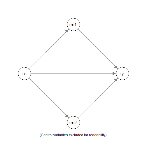
We would to fit the model above, and compute and test the indirect effects along the paths fx -> fm1 -> y and fx -> fm2 -> y using nonparametric bootstrapping.

Analysis

We can do that in one single step using q_parallel_mediation():

out <- q_parallel_mediation(
  x = "fx",
  y = "fy",
  m = c("fm1", "fm2"),
  cov = c("fc1", "c2"),
  indicators = list(
    fx = c("x_1", "x_2", "x_3", "-x_4"),
    fy = c("y_1", "y_2", "y_3", "-y_4"),
    fm1 = c("m1_1", "m1_2", "m1_3", "m1_4"),
    fm2 = c("m2_1", "m2_2", "m2_3", "m2_4"),
    fc1 = c("c1_1", "c1_2", "c1_3", "c1_4")
  ),
  fit_method = "sem",
  indicator_method = "measurement_model",
  data = dat,
  R = 5000,
  seed = 1234
)

These are the arguments:

x: The name of the predictor (“x” variable).
y: The name of the outcome (“y” variable).
m: A vector of the names of the mediators (“m” variables). For a parallel mediation model, the order of the mediators does not matter.
cov: The name(s) of the control variable(s) (covariate(s)). By default, they predict both the mediator and the outcome.
indicators: The indicators for latent variables. It should be a named list of variable names. The name of each element is the name of the latent variable. If an indicator is a reverse item, add a minus sign, -, before its name. It will be reverse-coded (multiplied by -1) before fitting the model. If a variable in x, y, m, or cov is not one of the latent factor, it is an observed variable.
fit_method and indicator_method: To fit a model with the measurement part, using the information from indicators, set fit_method to "sem" and indicator_method to "measurement_model"
data: The data frame for the model.
R: The number of bootstrap samples. Should be at least 5000 but can be larger for stable results.
seed: The seed for the random number generator. Should always be set to an integer to make the results reproducible.

The computation may take some time to run, especially if missing data is presence, due to the processing time combining bootstrapping and full-information maximum likelihood (FIML), the default way to handle missing data.

Results

We can then just print the output:

out

The printout is long. They will be discussed section-by-section below.

These are the main sections of the default results:

Basic Information

This is the section Basic Information:

#> ===================================================
#> |                Basic Information                |
#> ===================================================
#> 
#> Predictor(x): fx
#> Outcome(y): fy
#> Mediator(s)(m): fm1, fm2
#> Model: Parallel Mediation Model
#> Indicators Method: Fit a measurement model
#> 
#> The path model fitted:
#> 
#> fm1 ~ fx + fc1 + c2
#> fm2 ~ fx + fc1 + c2
#> fy ~ fm1 + fm2 + fx + fc1 + c2
#> fx =~ x_1 + x_2 + x_3 + x_4
#> fy =~ y_1 + y_2 + y_3 + y_4
#> fm1 =~ m1_1 + m1_2 + m1_3 + m1_4
#> fm2 =~ m2_1 + m2_2 + m2_3 + m2_4
#> fc1 =~ c1_1 + c1_2 + c1_3 + c1_4 
#> 
#> The original number of cases: 600 
#> The number of cases in the analysis: 600 
#> Missing data handling: FIML (full information maximum likelihood)

It shows the variables, the models, and the number of cases. It also shows the measurement model in the model, in lavaan syntax:

The name on the left-hand side of =~ is the latent variable.
The name on the right-hand side of =~, joined by +, are the indicators.

When the model is fitted by SEM, the default method to handle missing data is full-information maximum likelihood (FIML).

Indicator Information

#> ===================================================
#> |              Indicator Information              |
#> ===================================================
#> 
#> The indicators for the following variable(s):
#> 
#> fx: x_1, x_2, x_3, -x_4
#> fy: y_1, y_2, y_3, -y_4
#> fm1: m1_1, m1_2, m1_3, m1_4
#> fm2: m2_1, m2_2, m2_3, m2_4
#> fc1: c1_1, c1_2, c1_3, c1_4
#> 
#> Note:
#> - '-' denotes revserse-coded items.
#> 
#> The standardized factor loadings:
#> 
#> fx: 
#> Reliability: 0.7216
#>     Loading
#> x_1  0.5675
#> x_2  0.5902
#> x_3  0.6654
#> x_4  0.6802
#> 
#> fy: 
#> Reliability: 0.8812
#>     Loading
#> y_1  0.8308
#> y_2  0.7786
#> y_3  0.8039
#> y_4  0.8097
#> 
#> fm1: 
#> Reliability: 0.7751
#>      Loading
#> m1_1  0.6904
#> m1_2  0.6282
#> m1_3  0.7205
#> m1_4  0.6742
#> 
#> fm2: 
#> Reliability: 0.6630
#>      Loading
#> m2_1  0.6081
#> m2_2  0.5265
#> m2_3  0.5432
#> m2_4  0.6160
#> 
#> fc1: 
#> Reliability: 0.7149
#>      Loading
#> c1_1  0.6034
#> c1_2  0.6588
#> c1_3  0.5558
#> c1_4  0.6608
#> 
#> Note:
#> - Revserse-coded items have been reverse-coded when estimating the
#>   loadings.
#> - If the loading of an item is negative, its coding (revserse or
#>   non-reverse) may be incorrect.
#> - Reliability estimated by omage coefficients.

The section Indicator Information shows results related to each latent factor:

The indicators for each latent variable.
The standardized factor loadings from the SEM results.
- Note that, after recoding, all loadings should be positive. If any loading is negative, it may be a reverse indicator not specified in indicators.
The reliability coefficient for each latent factor, based on the factor loadings. Omega coefficient is used, computed by semTools::compRelSEM().

Model Fit

The section Structural Equation Modeling Results print the results from lavaan for the model.

#> Model Test User Model:
#>                                                       
#>   Test statistic                               175.086
#>   Degrees of freedom                               178
#>   P-value (Chi-square)                           0.548
#> 
#> Model Test Baseline Model:
#> 
#>   Test statistic                              3674.693
#>   Degrees of freedom                               210
#>   P-value                                        0.000
#> 
#> User Model versus Baseline Model:
#> 
#>   Comparative Fit Index (CFI)                    1.000
#>   Tucker-Lewis Index (TLI)                       1.001
#> 
#> Root Mean Square Error of Approximation:
#> 
#>   RMSEA                                          0.000
#>   Confidence interval - lower                    0.000
#>   Confidence interval - upper                    0.017
#>   P-value H_0: RMSEA <= 0.050                    1.000
#>   P-value H_0: RMSEA >= 0.080                    0.000
#> 
#> Standardized Root Mean Square Residual:
#> 
#>   SRMR                                           0.030

First, results on goodness-of-fit are printed:

Model Test User Model reports the model $\chi^2$ and its df and p-value.
Basic fit measures (CFI, TLI, RMSEA, and SRMR) are also printed.

Regression Results

The next few sections print the regression coefficients when predicting the mediators (fm1 and fm2 in this model) and the outcome variable (fy in this model).

These are the results in predicting fm1 and fm2:

#>  ---------------- 
#>  Predicting fm1 : 
#>  ---------------- 
#> 
#> Model:
#>  fm1 ~ fx + fc1 + c2 
#>             Estimate   CI.lo   CI.hi   betaS Std. Error z value Pr(>|z|)    
#> (Intercept)   0.0000  0.0000  0.0000    ----     0.0000    ----     ----    
#> fx            0.6759  0.4757  0.8761  0.4839     0.1021   6.618   <2e-16 ***
#> fc1           0.0795 -0.0778  0.2368  0.0601     0.0803   0.990    0.322    
#> c2            0.0455 -0.0462  0.1371  0.0421     0.0468   0.972    0.331    
#> ---
#> Signif. codes:  0 '***' 0.001 '**' 0.01 '*' 0.05 '.' 0.1 ' ' 1
#> 
#> R-square:  0.2653 
#> 
#> Chi-Squared Difference Test for the R-square
#> 
#>       Df   AIC   BIC  Chisq Chisq diff Df diff Pr(>Chisq)    
#> fit1 178 38135 38451 175.09                                  
#> fit0 181 38234 38537 280.27     105.18       3  < 2.2e-16 ***
#> ---
#> Signif. codes:  0 '***' 0.001 '**' 0.01 '*' 0.05 '.' 0.1 ' ' 1
#> 
#> - BetaS are standardized coefficients with (a) only numeric variables
#>   standardized and (b) product terms formed after standardization.
#>   Variable(s) standardized is/are: fm1, fx, fc1, c2
#> - CI.lo and CI.hi are the 95.0% confidence levels of 'Estimate'
#>   computed from the z values and standard errors.
#> 
#>  ---------------- 
#>  Predicting fm2 : 
#>  ---------------- 
#> 
#> Model:
#>  fm2 ~ fx + fc1 + c2 
#>             Estimate   CI.lo   CI.hi   betaS Std. Error z value Pr(>|z|)    
#> (Intercept)   0.0000  0.0000  0.0000    ----     0.0000    ----     ----    
#> fx            0.4583  0.2944  0.6222  0.4271     0.0836   5.480   <2e-16 ***
#> fc1           0.0525 -0.0808  0.1858  0.0517     0.0680   0.772    0.440    
#> c2            0.0442 -0.0342  0.1226  0.0533     0.0400   1.106    0.269    
#> ---
#> Signif. codes:  0 '***' 0.001 '**' 0.01 '*' 0.05 '.' 0.1 ' ' 1
#> 
#> R-square:  0.2075 
#> 
#> Chi-Squared Difference Test for the R-square
#> 
#>       Df   AIC   BIC  Chisq Chisq diff Df diff Pr(>Chisq)    
#> fit1 178 38135 38451 175.09                                  
#> fit0 181 38198 38502 244.81     69.721       3  4.897e-15 ***
#> ---
#> Signif. codes:  0 '***' 0.001 '**' 0.01 '*' 0.05 '.' 0.1 ' ' 1
#> 
#> - BetaS are standardized coefficients with (a) only numeric variables
#>   standardized and (b) product terms formed after standardization.
#>   Variable(s) standardized is/are: fm2, fx, fc1, c2
#> - CI.lo and CI.hi are the 95.0% confidence levels of 'Estimate'
#>   computed from the z values and standard errors.

These are the results in predicting y:

#>  --------------- 
#>  Predicting fy : 
#>  --------------- 
#> 
#> Model:
#>  fy ~ fm1 + fm2 + fx + fc1 + c2 
#>             Estimate   CI.lo   CI.hi   betaS Std. Error z value Pr(>|z|)    
#> (Intercept)   0.0000  0.0000  0.0000    ----     0.0000    ----     ----    
#> fm1           0.5005  0.3488  0.6522  0.3546     0.0774   6.466   <2e-16 ***
#> fm2           0.5904  0.3818  0.7990  0.3213     0.1064   5.547   <2e-16 ***
#> fx            0.2035 -0.0553  0.4622  0.1032     0.1320   1.541   0.1233    
#> fc1           0.3114  0.1253  0.4975  0.1670     0.0949   3.280   0.0010 ***
#> c2            0.1349  0.0264  0.2433  0.0884     0.0553   2.437   0.0148 *  
#> ---
#> Signif. codes:  0 '***' 0.001 '**' 0.01 '*' 0.05 '.' 0.1 ' ' 1
#> 
#> R-square:  0.4751 
#> 
#> Chi-Squared Difference Test for the R-square
#> 
#>       Df   AIC   BIC  Chisq Chisq diff Df diff Pr(>Chisq)    
#> fit1 178 38135 38451 175.09                                  
#> fit0 183 38387 38682 437.86     262.78       5  < 2.2e-16 ***
#> ---
#> Signif. codes:  0 '***' 0.001 '**' 0.01 '*' 0.05 '.' 0.1 ' ' 1
#> 
#> - BetaS are standardized coefficients with (a) only numeric variables
#>   standardized and (b) product terms formed after standardization.
#>   Variable(s) standardized is/are: fy, fm1, fm2, fx, fc1, c2
#> - CI.lo and CI.hi are the 95.0% confidence levels of 'Estimate'
#>   computed from the z values and standard errors.

The results from lavaan::sem() are reformatted to make them similar to those by regression analysis.

If desired, the output of lavaan::sem() can be extracted from the output by get_fit().

Indirect Effect Results

By default, this section prints the estimated indirect effect, confidence interval, and asymmetric bootstrap p-value.

Four sections will be printed:

The original indirect effect.

#> == Indirect Effect(s) ==
#> 
#>                    ind  CI.lo  CI.hi Sig pvalue     SE
#> fx -> fm1 -> fy 0.3383 0.2231 0.4808 Sig 0.0000 0.0663
#> fx -> fm2 -> fy 0.2705 0.1586 0.4138 Sig 0.0000 0.0657
#> 
#>  - [CI.lo to CI.hi] are 95.0% percentile confidence intervals by
#>    nonparametric bootstrapping with 5000 samples.
#>  - [pvalue] are asymmetric bootstrap p-values.
#>  - [SE] are standard errors.
#>  - The 'ind' column shows the indirect effect(s).

The indirect effect with the predictor (“x”) standardized.

#> == Indirect Effect(s) (x-variable(s) Standardized) ==
#> 
#>                    std  CI.lo  CI.hi Sig pvalue     SE
#> fx -> fm1 -> fy 0.2426 0.1621 0.3362 Sig 0.0000 0.0440
#> fx -> fm2 -> fy 0.1940 0.1152 0.2920 Sig 0.0000 0.0455
#> 
#>  - [CI.lo to CI.hi] are 95.0% percentile confidence intervals by
#>    nonparametric bootstrapping with 5000 samples.
#>  - [pvalue] are asymmetric bootstrap p-values.
#>  - [SE] are standard errors.
#>  - std: The partially standardized indirect effect(s).
#>  - x-variable(s) standardized.

The indirect effect with the outcome (“y”) standardized.

#> == Indirect Effect(s) (y-variable(s) Standardized) ==
#> 
#>                    std  CI.lo  CI.hi Sig pvalue     SE
#> fx -> fm1 -> fy 0.2393 0.1586 0.3385 Sig 0.0000 0.0471
#> fx -> fm2 -> fy 0.1914 0.1140 0.2932 Sig 0.0000 0.0455
#> 
#>  - [CI.lo to CI.hi] are 95.0% percentile confidence intervals by
#>    nonparametric bootstrapping with 5000 samples.
#>  - [pvalue] are asymmetric bootstrap p-values.
#>  - [SE] are standard errors.
#>  - std: The partially standardized indirect effect(s).
#>  - y-variable(s) standardized.

The indirect effect with both x and y standardized.

#> == Indirect Effect(s) (Both x-variable(s) and y-variable(s) Standardized) ==
#> 
#>                    std  CI.lo  CI.hi Sig pvalue     SE
#> fx -> fm1 -> fy 0.1716 0.1152 0.2375 Sig 0.0000 0.0310
#> fx -> fm2 -> fy 0.1372 0.0820 0.2057 Sig 0.0000 0.0314
#> 
#>  - [CI.lo to CI.hi] are 95.0% percentile confidence intervals by
#>    nonparametric bootstrapping with 5000 samples.
#>  - [pvalue] are asymmetric bootstrap p-values.
#>  - [SE] are standard errors.
#>  - std: The standardized indirect effect(s).

The indirect effect with both the predictor (“x”) and the outcome (“y”) standardized, also called the completely standardized indirect effect or simply the standardized indirect effect.

These four versions of the results are printed by default so that users can select and interpret sections as they see fit.

Total Indirect Effect Results

The section Total Indirect Effects Results prints the estimated total indirect effects, confidence intervals, and asymmetric bootstrap p-values.

#> ===================================================
#> |          Total Indirect Effect Results          |
#> ===================================================
#> 
#> ----------------------------------------------------------------
#> 
#> == Indirect Effect  ==
#>                                         
#>  Path:                fx -> fm1 -> fy   
#>  Path:                fx -> fm2 -> fy   
#>  Function of Effects: 0.6088            
#>  95.0% Bootstrap CI:  [0.4365 to 0.8299]
#>  Bootstrap p-value:   0.0000            
#>  Bootstrap SE:        0.0998            
#> 
#> Computation of the Function of Effects:
#>  (fx->fm1->fy)
#> +(fx->fm2->fy) 
#> 
#> 
#> Percentile confidence interval formed by nonparametric bootstrapping
#> with 5000 bootstrap samples.
#> Standard error (SE) based on nonparametric bootstrapping with 5000
#> bootstrap samples.
#> 
#> 
#> ----------------------------------------------------------------
#> 
#> == Indirect Effect ('fx' Standardized) ==
#>                                         
#>  Path:                fx -> fm1 -> fy   
#>  Path:                fx -> fm2 -> fy   
#>  Function of Effects: 0.4366            
#>  95.0% Bootstrap CI:  [0.3187 to 0.5735]
#>  Bootstrap p-value:   0.0000            
#>  Bootstrap SE:        0.0656            
#> 
#> Computation of the Function of Effects:
#>  (fx->fm1->fy)
#> +(fx->fm2->fy) 
#> 
#> 
#> Percentile confidence interval formed by nonparametric bootstrapping
#> with 5000 bootstrap samples.
#> Standard error (SE) based on nonparametric bootstrapping with 5000
#> bootstrap samples.
#> 
#> 
#> ----------------------------------------------------------------
#> 
#> == Indirect Effect ('fy' Standardized) ==
#>                                         
#>  Path:                fx -> fm1 -> fy   
#>  Path:                fx -> fm2 -> fy   
#>  Function of Effects: 0.4307            
#>  95.0% Bootstrap CI:  [0.3114 to 0.5811]
#>  Bootstrap p-value:   0.0000            
#>  Bootstrap SE:        0.0693            
#> 
#> Computation of the Function of Effects:
#>  (fx->fm1->fy)
#> +(fx->fm2->fy) 
#> 
#> 
#> Percentile confidence interval formed by nonparametric bootstrapping
#> with 5000 bootstrap samples.
#> Standard error (SE) based on nonparametric bootstrapping with 5000
#> bootstrap samples.
#> 
#> 
#> ----------------------------------------------------------------
#> 
#> == Indirect Effect (Both 'fx' and 'fy' Standardized) ==
#>                                         
#>  Path:                fx -> fm1 -> fy   
#>  Path:                fx -> fm2 -> fy   
#>  Function of Effects: 0.3089            
#>  95.0% Bootstrap CI:  [0.2266 to 0.4022]
#>  Bootstrap p-value:   0.0000            
#>  Bootstrap SE:        0.0449            
#> 
#> Computation of the Function of Effects:
#>  (fx->fm1->fy)
#> +(fx->fm2->fy) 
#> 
#> 
#> Percentile confidence interval formed by nonparametric bootstrapping
#> with 5000 bootstrap samples.
#> Standard error (SE) based on nonparametric bootstrapping with 5000
#> bootstrap samples.

The total indirect effect in a parallel mediation model is the sum of all indirect effects from the predictor (“x”) to the outcome (“y”).

Four sections will be printed:

The original total indirect effect.
The total indirect effects with the predictor (“x”) standardized.
The total indirect effects with the outcome (“y”) standardized.
The total indirect effects with both the predictor (“x”) and the outcome (“y”) standardized, also called the completely standardized total indirect effects or simply the standardized total indirect effects.

These four versions of the results are printed by default such that users can select and interpret sections as they see fit.

Direct Effect Results

The section Direct Effect Results prints the estimated direct effect (from the predictor “x” to the outcome “y”, not mediated), confidence interval, and asymmetric bootstrap p-value.

#> ===================================================
#> |              Direct Effect Results              |
#> ===================================================
#> 
#> ----------------------------------------------------------------
#> 
#> == Effect(s) ==
#> 
#>             ind   CI.lo  CI.hi Sig pvalue     SE
#> fx -> fy 0.2035 -0.0640 0.4823     0.1348 0.1399
#> 
#>  - [CI.lo to CI.hi] are 95.0% percentile confidence intervals by
#>    nonparametric bootstrapping with 5000 samples.
#>  - [pvalue] are asymmetric bootstrap p-values.
#>  - [SE] are standard errors.
#>  - The 'ind' column shows the effect(s).
#>  
#> ----------------------------------------------------------------
#> 
#> == Effect(s) (x-variable(s) Standardized) ==
#> 
#>             std   CI.lo  CI.hi Sig pvalue     SE
#> fx -> fy 0.1459 -0.0473 0.3389     0.1348 0.0984
#> 
#>  - [CI.lo to CI.hi] are 95.0% percentile confidence intervals by
#>    nonparametric bootstrapping with 5000 samples.
#>  - [pvalue] are asymmetric bootstrap p-values.
#>  - [SE] are standard errors.
#>  - std: The partially standardized effect(s).
#>  - x-variable(s) standardized.
#>  
#> ----------------------------------------------------------------
#> 
#> == Effect(s) (y-variable(s) Standardized) ==
#> 
#>             std   CI.lo  CI.hi Sig pvalue     SE
#> fx -> fy 0.1439 -0.0486 0.3402     0.1348 0.0989
#> 
#>  - [CI.lo to CI.hi] are 95.0% percentile confidence intervals by
#>    nonparametric bootstrapping with 5000 samples.
#>  - [pvalue] are asymmetric bootstrap p-values.
#>  - [SE] are standard errors.
#>  - std: The partially standardized effect(s).
#>  - y-variable(s) standardized.
#>  
#> ----------------------------------------------------------------
#> 
#> == Effect(s) (Both x-variable(s) and y-variable(s) Standardized) ==
#> 
#>             std   CI.lo  CI.hi Sig pvalue     SE
#> fx -> fy 0.1032 -0.0335 0.2390     0.1348 0.0695
#> 
#>  - [CI.lo to CI.hi] are 95.0% percentile confidence intervals by
#>    nonparametric bootstrapping with 5000 samples.
#>  - [pvalue] are asymmetric bootstrap p-values.
#>  - [SE] are standard errors.

The z-test of the direct effect is already available in section Structural Equation Modeling Results. The bootstrap results are printed in case users prefer using the same confidence interval method for all the effects.

Additional Issues

Customize Control Variables

If the control variables for the regression models are different, we can set cov to a named list. The names are the variables with control variables, and the element under each name is a character vector of the control variables.

For example,

If we set cov to list(m1 = "c1", m2 = "c2", y = c("c1", "c2")), then only c1 is included in predicting m1, only c2 is included in predicting m2, while both c1 and c2 are included in predicting y.

A variable that does not appear in the list does not have control variables.

Customize The Printout

The print method of the output of the quick mediation functions have arguments for customizing the output. These are arguments that likely may be used:

digits: The number of digits after the decimal place for most results. Default is 4.
pvalue_digits: The number of digits after the decimal place for p-values. Default is 4.

See the help page of print.q_mediation() for other arguments.

Speed and Parallel Processing

By default, parallel processing is used. If this failed for some reasons, add parallel to FALSE. It will take longer, sometimes much long, to run if parallel is set to FALSE. Therefore, use parallel processing whenever possible.

Progress Bar

By default, a progress bar will be displayed when doing bootstrapping. This can be disabled by adding progress = FALSE.

Workflow

The quick functions are simply functions to do the following tasks internally:

Fit all the models by SEM using lavaan::sem().
Call all_indirect_paths() to identify all indirect paths.
Call many_indirect_effects() to compute all indirect effects and form their confidence intervals.
Call total_indirect_effect() to compute the total indirect effect.

Therefore, all the tasks they do can be done manually by the functions above. These all-in-one functions are developed just as convenient functions to do all these tasks in one call.

See this article for computing and testing indirect effects for more complicated models.

Final Remarks

For details on the all-in-one functions, please refer to the help page of q_mediation().

Using `q_mediation()`

Shu Fai Cheung & Sing-Hang Cheung

2026-05-28

Introduction

Data Set

Parallel Mediation Model

Analysis

Results

Basic Information

Indicator Information

Model Fit

Regression Results

Indirect Effect Results

Total Indirect Effect Results

Direct Effect Results

Additional Issues

Customize Control Variables

Customize The Printout

Speed and Parallel Processing

Progress Bar

Workflow

Final Remarks

Parallel Mediation Models Corrected for Measurement Error

Using q_mediation()

Shu Fai Cheung & Sing-Hang Cheung

2026-05-28

Introduction

Data Set

Parallel Mediation Model

Analysis

Results

Basic Information

Indicator Information

Model Fit

Regression Results

Indirect Effect Results

Total Indirect Effect Results

Direct Effect Results

Additional Issues

Customize Control Variables

Customize The Printout

Speed and Parallel Processing

Progress Bar

Workflow

Final Remarks

Using `q_mediation()`