Multigroup Models With Mediation Effects
Shu Fai Cheung & Sing-Hang Cheung
2026-03-26
Source:vignettes/articles/med_mg.Rmd
med_mg.RmdIntroduction
This article is a brief illustration of how to use manymome (Cheung & Cheung,
2024) to compute and test indirect effects in a multigroup model
fitted by lavaan. 1
This article only focuses on issues specific to multigroup models.
Readers are assumed to have basic understanding on using
manymome. Please refer to the Get
Started guide for a full introduction, and this
section on an illustration on a mediation model.
Model
This is the sample data set that comes with the package:
library(manymome)
dat <- data_med_mg
print(head(dat), digits = 3)
#> x m y c1 c2 group
#> 1 10.11 17.0 17.4 1.9864 5.90 Group A
#> 2 9.75 16.6 17.5 0.7748 4.37 Group A
#> 3 9.81 17.9 14.9 0.0973 6.96 Group A
#> 4 10.15 19.7 18.0 2.3974 5.75 Group A
#> 5 10.30 17.7 20.7 3.2225 5.84 Group A
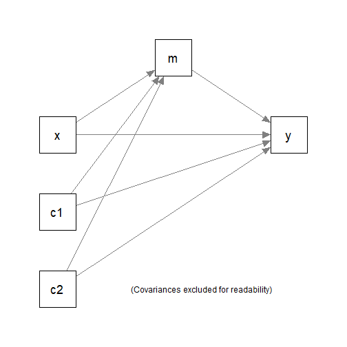
#> 6 10.01 18.9 20.7 2.3631 4.51 Group ASuppose this is the model being fitted, with c1 and
c2 the control variables. The grouping variable is
group, with two possible values, "Group A" and
"Group B".
Fitting the Model
We first fit this multigroup model in lavaan::sem() as
usual. There is no need to label any parameters because
manymome will extract the parameters automatically.
mod_med <-
"
m ~ x + c1 + c2
y ~ m + x + c1 + c2
"
fit <- sem(model = mod_med,
           data = dat,
           fixed.x = FALSE,
           group = "group")
These are the estimates of the paths:
summary(fit,
        estimates = TRUE)
#> lavaan 0.6-21 ended normally after 1 iteration
#>
#>   Estimator                                         ML
#>   Optimization method                           NLMINB
#>   Number of model parameters                        40
#>
#>   Number of observations per group:
#>     Group A                                        100
#>     Group B                                        150
#>
#> Model Test User Model:
#>
#>   Test statistic                                 0.000
#>   Degrees of freedom                                 0
#>   Test statistic for each group:
#>     Group A                                      0.000
#>     Group B                                      0.000
#>
#> Parameter Estimates:
#>
#>   Standard errors                             Standard
#>   Information                                 Expected
#>   Information saturated (h1) model          Structured
#>
#>
#> Group 1 [Group A]:
#>
#> Regressions:
#>                    Estimate  Std.Err  z-value  P(>|z|)
#>   m ~
#>     x                 0.880    0.093    9.507    0.000
#>     c1                0.264    0.104    2.531    0.011
#>     c2               -0.316    0.095   -3.315    0.001
#>   y ~
#>     m                 0.465    0.190    2.446    0.014
#>     x                 0.321    0.243    1.324    0.186
#>     c1                0.285    0.204    1.395    0.163
#>     c2               -0.228    0.191   -1.195    0.232
#>
#> Covariances:
#>                    Estimate  Std.Err  z-value  P(>|z|)
#>   x ~~
#>     c1               -0.080    0.107   -0.741    0.459
#>     c2               -0.212    0.121   -1.761    0.078
#>   c1 ~~
#>     c2               -0.071    0.104   -0.677    0.499
#>
#> Intercepts:
#>                    Estimate  Std.Err  z-value  P(>|z|)
#>    .m                10.647    1.156    9.211    0.000
#>    .y                 6.724    2.987    2.251    0.024
#>     x                 9.985    0.111   90.313    0.000
#>     c1                2.055    0.097   21.214    0.000
#>     c2                4.883    0.107   45.454    0.000
#>
#> Variances:
#>                    Estimate  Std.Err  z-value  P(>|z|)
#>    .m                 1.006    0.142    7.071    0.000
#>    .y                 3.633    0.514    7.071    0.000
#>     x                 1.222    0.173    7.071    0.000
#>     c1                0.939    0.133    7.071    0.000
#>     c2                1.154    0.163    7.071    0.000
#>
#>
#> Group 2 [Group B]:
#>
#> Regressions:
#>                    Estimate  Std.Err  z-value  P(>|z|)
#>   m ~
#>     x                 0.597    0.081    7.335    0.000
#>     c1                0.226    0.087    2.610    0.009
#>     c2               -0.181    0.078   -2.335    0.020
#>   y ~
#>     m                 1.110    0.171    6.492    0.000
#>     x                 0.264    0.199    1.330    0.183
#>     c1               -0.016    0.186   -0.088    0.930
#>     c2               -0.072    0.165   -0.437    0.662
#>
#> Covariances:
#>                    Estimate  Std.Err  z-value  P(>|z|)
#>   x ~~
#>     c1                0.102    0.079    1.299    0.194
#>     c2               -0.050    0.087   -0.574    0.566
#>   c1 ~~
#>     c2                0.109    0.083    1.313    0.189
#>
#> Intercepts:
#>                    Estimate  Std.Err  z-value  P(>|z|)
#>    .m                 7.862    0.924    8.511    0.000
#>    .y                 1.757    2.356    0.746    0.456
#>     x                10.046    0.082  121.888    0.000
#>     c1                2.138    0.078   27.515    0.000
#>     c2                5.088    0.087   58.820    0.000
#>
#> Variances:
#>                    Estimate  Std.Err  z-value  P(>|z|)
#>    .m                 0.998    0.115    8.660    0.000
#>    .y                 4.379    0.506    8.660    0.000
#>     x                 1.019    0.118    8.660    0.000
#>     c1                0.906    0.105    8.660    0.000
#>     c2                1.122    0.130    8.660    0.000
Generate Bootstrap estimates
We can use do_boot() to generate the bootstrap estimates
first (see this
article for an illustration on this function). The argument
ncores can be omitted if the default value is
acceptable.
fit_boot_out <- do_boot(fit = fit,
                        R = 5000,
                        seed = 53253,
                        ncores = 8)
#> 8 processes started to run bootstrapping.
Estimate Indirect Effects
Estimate Each Effect by indirect_effect()
The function indirect_effect() can be used to as usual
to estimate an indirect effect and form its bootstrapping or Monte Carlo
confidence interval along a path in a model that starts with any numeric
variable, ends with any numeric variable, through any numeric
variable(s). A detailed illustration can be found in this
section.
For a multigroup model, the only difference is that users need to
specify the group using the argument group. It can be set
to the group label as used in lavaan
("Group A" or "Group B" in this example) or
the group number used in lavaan
ind_gpA <- indirect_effect(x = "x",
                           y = "y",
                           m = "m",
                           fit = fit,
                           group = "Group A",
                           boot_ci = TRUE,
                           boot_out = fit_boot_out)
This is the output:
ind_gpA
#>
#> == Indirect Effect  ==
#>
#>  Path:               Group A[1]: x -> m -> y
#>  Indirect Effect:    0.409
#>  95.0% Bootstrap CI: [0.096 to 0.753]
#>
#> Computation Formula:
#>   (b.m~x)*(b.y~m)
#>
#> Computation:
#>   (0.87989)*(0.46481)
#>
#>
#> Percentile confidence interval formed by nonparametric bootstrapping
#> with 5000 bootstrap samples.
#>
#> Coefficients of Component Paths:
#>  Path Coefficient
#>   m~x       0.880
#>   y~m       0.465
#>
#> NOTE:
#> - The group label is printed before each path.
#> - The group number in square brackets is the number used internally in
#>   lavaan.
The indirect effect from x to y through
m in "Group A" is 0.409, with a 95% confidence
interval of [0.096, 0.753], significantly different from zero
(p < .05).
We illustrate computing the indirect effect in
"Group B", using group number:
ind_gpB <- indirect_effect(x = "x",
                           y = "y",
                           m = "m",
                           fit = fit,
                           group = 2,
                           boot_ci = TRUE,
                           boot_out = fit_boot_out)
This is the output:
ind_gpB
#>
#> == Indirect Effect  ==
#>
#>  Path:               Group B[2]: x -> m -> y
#>  Indirect Effect:    0.663
#>  95.0% Bootstrap CI: [0.411 to 0.959]
#>
#> Computation Formula:
#>   (b.m~x)*(b.y~m)
#>
#> Computation:
#>   (0.59716)*(1.11040)
#>
#>
#> Percentile confidence interval formed by nonparametric bootstrapping
#> with 5000 bootstrap samples.
#>
#> Coefficients of Component Paths:
#>  Path Coefficient
#>   m~x       0.597
#>   y~m       1.110
#>
#> NOTE:
#> - The group label is printed before each path.
#> - The group number in square brackets is the number used internally in
#>   lavaan.
The indirect effect from x to y through
m in "Group B" is 0.663, with a 95% confidence
interval of [0.096, 0.753], also significantly different from zero
(p < .05).
Treating Group as a “Moderator”
Instead of computing the indirect effects one-by-one, we can also
treat the grouping variable as a “moderator” and use
cond_indirect_effects() to compute the indirect effects
along a path for all groups. The detailed illustration of this function
can be found here.
When use on a multigroup model, wwe can omit the argument
wlevels. The function will automatically identify all
groups in a model, and compute the indirect effect of the requested path
in each model.
ind <- cond_indirect_effects(x = "x",
                             y = "y",
                             m = "m",
                             fit = fit,
                             boot_ci = TRUE,
                             boot_out = fit_boot_out)
This is the output:
ind
#>
#> == Conditional indirect effects ==
#>
#>  Path: x -> m -> y
#>  Conditional on group(s): Group A[1], Group B[2]
#>
#>     Group Group_ID   ind CI.lo CI.hi Sig   m~x   y~m
#> 1 Group A        1 0.409 0.096 0.753 Sig 0.880 0.465
#> 2 Group B        2 0.663 0.411 0.959 Sig 0.597 1.110
#>
#>  - [CI.lo to CI.hi] are 95.0% percentile confidence intervals by
#>    nonparametric bootstrapping with 5000 samples.
#>  - The 'ind' column shows the indirect effects.
#>  - 'm~x','y~m' is/are the path coefficient(s) along the path conditional
#>    on the group(s).
The results are identical to those computed individually using
indirect_effect(). Using
cond_indirect_effects() is convenient when the number of
groups is more than two.
Compute and Test Between-Group difference
There are several ways to compute and test the difference in indirect effects between two groups.
Using the Math Operator -
The math operator - (described here)
can be used if the indirect effects have been computed individually by
indirect_effect(). We have already computed the path
x->m->y before for the two groups. Let us compute the
differences:
ind_diff <- ind_gpB - ind_gpA
ind_diff
#>
#> == Indirect Effect  ==
#>
#>  Path:                Group B[2]: x -> m -> y
#>  Path:                Group A[1]: x -> m -> y
#>  Function of Effects: 0.254
#>  95.0% Bootstrap CI:  [-0.173 to 0.685]
#>
#> Computation of the Function of Effects:
#>  (Group B[2]: x->m->y)
#> -(Group A[1]: x->m->y)
#>
#>
#> Percentile confidence interval formed by nonparametric bootstrapping
#> with 5000 bootstrap samples.
#>
#> NOTE:
#> - The group label is printed before each path.
#> - The group number in square brackets is the number used internally in
#>   lavaan.
The difference in indirect effects from x to
y through m is 0.254, with a 95% confidence
interval of [-0.173, 0.685], not significantly different from zero
(p < .05). Therefore, we conclude that the two groups are
not significantly different on the indirect effects.
Using cond_indirect_diff()
If the indirect effects are computed using
cond_indirect_effects(), we can use the function
cond_indirect_diff() to compute the difference (described
here)
This is more convenient than using the math operator when the number of
groups is greater than two.
Let us use cond_indirect_diff() on the output of
cond_indirect_effects():
ind_diff2 <- cond_indirect_diff(ind,
                                from = 1,
                                to = 2)
ind_diff2
#>
#> == Conditional indirect effects ==
#>
#>  Path: x -> m -> y
#>  Conditional on group(s): Group B[2], Group A[1]
#>
#>     Group Group_ID   ind CI.lo CI.hi Sig   m~x   y~m
#> 1 Group B        2 0.663 0.411 0.959 Sig 0.597 1.110
#> 2 Group A        1 0.409 0.096 0.753 Sig 0.880 0.465
#>
#> == Difference in Conditional Indirect Effect ==
#>
#> Levels:
#>        Group
#> To:    Group B [2]
#> From:  Group A [1]
#>
#> Levels compared: Group B [2] - Group A [1]
#>
#> Change in Indirect Effect:
#>
#>        x y Change  CI.lo CI.hi
#> Change x y  0.254 -0.173 0.685
#>
#>  - [CI.lo, CI.hi]: 95% percentile confidence interval.
The convention is to row minus from row.
Though may sound not intuitive, the printout always states clearly which
group is subtracted from which group. The results are identical to those
using the math operator.
Advanced Skills
Standardized Indirect Effects
Standardized indirect effects can be computed as for single-group
models (described here),
by setting standardized_x and/or
standardized_y. This is an example:
std_gpA <- indirect_effect(x = "x",
                           y = "y",
                           m = "m",
                           fit = fit,
                           group = "Group A",
                           boot_ci = TRUE,
                           boot_out = fit_boot_out,
                           standardized_x = TRUE,
                           standardized_y = TRUE)
std_gpA
#>
#> == Indirect Effect (Both 'x' and 'y' Standardized) ==
#>
#>  Path:               Group A[1]: x -> m -> y
#>  Indirect Effect:    0.204
#>  95.0% Bootstrap CI: [0.049 to 0.366]
#>
#> Computation Formula:
#>   (b.m~x)*(b.y~m)*sd_x/sd_y
#>
#> Computation:
#>   (0.87989)*(0.46481)*(1.10557)/(2.21581)
#>
#>
#> Percentile confidence interval formed by nonparametric bootstrapping
#> with 5000 bootstrap samples.
#>
#> Coefficients of Component Paths:
#>  Path Coefficient
#>   m~x       0.880
#>   y~m       0.465
#>
#> NOTE:
#> - The effects of the component paths are from the model, not
#>   standardized.
#> - SD(s) in the selected group is/are used in standardiziation.
#> - The group label is printed before each path.
#> - The group number in square brackets is the number used internally in
#>   lavaan.
std_gpB <- indirect_effect(x = "x",
                           y = "y",
                           m = "m",
                           fit = fit,
                           group = "Group B",
                           boot_ci = TRUE,
                           boot_out = fit_boot_out,
                           standardized_x = TRUE,
                           standardized_y = TRUE)
std_gpB
#>
#> == Indirect Effect (Both 'x' and 'y' Standardized) ==
#>
#>  Path:               Group B[2]: x -> m -> y
#>  Indirect Effect:    0.259
#>  95.0% Bootstrap CI: [0.166 to 0.360]
#>
#> Computation Formula:
#>   (b.m~x)*(b.y~m)*sd_x/sd_y
#>
#> Computation:
#>   (0.59716)*(1.11040)*(1.00943)/(2.58386)
#>
#>
#> Percentile confidence interval formed by nonparametric bootstrapping
#> with 5000 bootstrap samples.
#>
#> Coefficients of Component Paths:
#>  Path Coefficient
#>   m~x       0.597
#>   y~m       1.110
#>
#> NOTE:
#> - The effects of the component paths are from the model, not
#>   standardized.
#> - SD(s) in the selected group is/are used in standardiziation.
#> - The group label is printed before each path.
#> - The group number in square brackets is the number used internally in
#>   lavaan.
In "Group A", the (completely) standardized indirect
effect from x to y through m is
0.204. In "Group B", this effect is 0.259.
Note that, unlike single-group model, in multigroup models, the
standardized indirect effect in a group uses the the standard deviations
of x- and y-variables in this group to do the
standardization. Therefore, two groups can have different unstandardized
effects on a path but similar standardized effects on the same path, or
have similar unstandardized effects on a path but different standardized
effects on this path. This is a known phenomenon in multigroup
structural equation model.
The difference in the two completely standardized indirect effects
can computed and tested using the math operator -:
std_diff <- std_gpB - std_gpA
std_diff
#>
#> == Indirect Effect (Both 'x' and 'y' Standardized) ==
#>
#>  Path:                Group B[2]: x -> m -> y
#>  Path:                Group A[1]: x -> m -> y
#>  Function of Effects: 0.055
#>  95.0% Bootstrap CI:  [-0.133 to 0.245]
#>
#> Computation of the Function of Effects:
#>  (Group B[2]: x->m->y)
#> -(Group A[1]: x->m->y)
#>
#>
#> Percentile confidence interval formed by nonparametric bootstrapping
#> with 5000 bootstrap samples.
#>
#> NOTE:
#> - The group label is printed before each path.
#> - The group number in square brackets is the number used internally in
#>   lavaan.
The difference in completely standardized indirect effects from
x to y through m is 0.055, with a
95% confidence interval of [-0.133, 0.245], not significantly different
from zero (p < .05). Therefore, we conclude that the two
groups are also not significantly different on the completely
standardized indirect effects.
The function cond_indirect_effects() and
cond_indirect_diff() can also be used with
standardization:
std <- cond_indirect_effects(x = "x",
                             y = "y",
                             m = "m",
                             fit = fit,
                             boot_ci = TRUE,
                             boot_out = fit_boot_out,
                             standardized_x = TRUE,
                             standardized_y = TRUE)
std
#>
#> == Conditional indirect effects ==
#>
#>  Path: x -> m -> y
#>  Conditional on group(s): Group A[1], Group B[2]
#>
#>     Group Group_ID   std CI.lo CI.hi Sig   m~x   y~m   ind
#> 1 Group A        1 0.204 0.049 0.366 Sig 0.880 0.465 0.409
#> 2 Group B        2 0.259 0.166 0.360 Sig 0.597 1.110 0.663
#>
#>  - [CI.lo to CI.hi] are 95.0% percentile confidence intervals by
#>    nonparametric bootstrapping with 5000 samples.
#>  - std: The standardized indirect effects.
#>  - ind: The unstandardized indirect effects.
#>  - 'm~x','y~m' is/are the path coefficient(s) along the path conditional
#>    on the group(s).
std_diff2 <- cond_indirect_diff(std,
                                from = 1,
                                to = 2)
std_diff2
#>
#> == Conditional indirect effects ==
#>
#>  Path: x -> m -> y
#>  Conditional on group(s): Group B[2], Group A[1]
#>
#>     Group Group_ID   std CI.lo CI.hi Sig   m~x   y~m   ind
#> 1 Group B        2 0.259 0.166 0.360 Sig 0.597 1.110 0.663
#> 2 Group A        1 0.204 0.049 0.366 Sig 0.880 0.465 0.409
#>
#> == Difference in Conditional Indirect Effect ==
#>
#> Levels:
#>        Group
#> To:    Group B [2]
#> From:  Group A [1]
#>
#> Levels compared: Group B [2] - Group A [1]
#>
#> Change in Indirect Effect:
#>
#>        x y Change  CI.lo CI.hi
#> Change x y  0.055 -0.133 0.245
#>
#>  - [CI.lo, CI.hi]: 95% percentile confidence interval.
#>  - x standardized.
#>  - y standardized.
The results, again, are identical to those using
indirect_effect() and the math operator -.
Finding All Indirect Paths in a Multigroup Model
Suppose a model which has more than one, or has many, indirect paths, is fitted to this dataset:
dat2 <- data_med_complicated_mg
print(head(dat2), digits = 2)
#>     m11   m12     m2     y1     y2    x1     x2    c1      c2   group
#> 1  1.05  1.17  0.514  0.063  1.027  1.82 -0.365 0.580 -0.3221 Group A
#> 2 -0.48  0.71  0.366 -1.278 -1.442  0.18 -0.012 0.620 -0.8751 Group A
#> 3 -1.18 -2.01 -0.044 -0.177  0.152  0.32 -0.403 0.257 -0.1078 Group A
#> 4  3.64  1.47 -0.815  1.309  0.052  0.98  0.139 0.054  1.2495 Group A
#> 5 -0.41 -0.38 -1.177 -0.151  0.255 -0.36 -1.637 0.275  0.0078 Group A
#> 6  0.18 -1.00 -0.119 -0.588  0.036 -0.53  0.349 0.618 -0.4073 Group A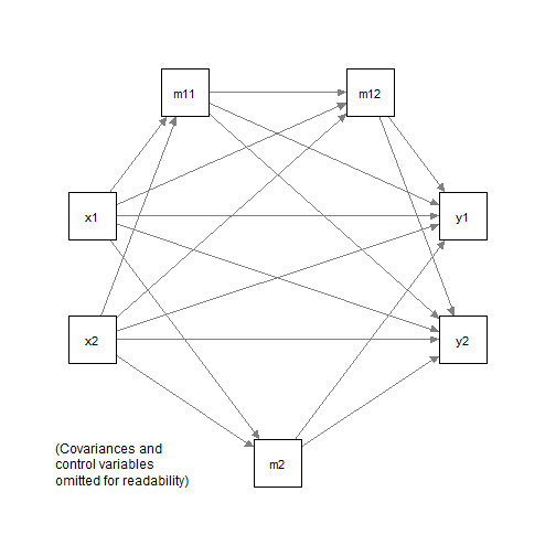
We first fit this model in lavaan:
mod2 <-
"
m11 ~ x1 + x2
m12 ~ m11 + x1 + x2
m2 ~ x1 + x2
y1 ~ m2 + m12 + m11 + x1 + x2
y2 ~ m2 + m12 + m11 + x1 + x2
"
fit2 <- sem(mod2, data = dat2, group = "group")
The function all_indirect_paths() can be used on a
multigroup model to identify indirect paths. The search can be
restricted by setting arguments such as x, y,
and exclude (see the help
page for details).
For example, the following identify all paths from x1 to
y1:
paths_x1_y1 <- all_indirect_paths(fit = fit2,
                                  x = "x1",
                                  y = "y1")
If the group argument is not specified, it will
automatically identify all paths in all groups, as shown in the
printout:
paths_x1_y1
#> Call:
#> all_indirect_paths(fit = fit2, x = "x1", y = "y1")
#> Path(s):
#>   path
#> 1 Group A.x1 -> m11 -> m12 -> y1
#> 2 Group A.x1 -> m11 -> y1
#> 3 Group A.x1 -> m12 -> y1
#> 4 Group A.x1 -> m2 -> y1
#> 5 Group B.x1 -> m11 -> m12 -> y1
#> 6 Group B.x1 -> m11 -> y1
#> 7 Group B.x1 -> m12 -> y1
#> 8 Group B.x1 -> m2 -> y1
We can then use many_indirect_effects() to compute the
indirect effects for all paths identified:
all_ind_x1_y1 <- many_indirect_effects(paths_x1_y1,
                                       fit = fit2)
all_ind_x1_y1
#>
#> == Indirect Effect(s) ==
#>
#>                                   ind
#> Group A.x1 -> m11 -> m12 -> y1  0.079
#> Group A.x1 -> m11 -> y1         0.106
#> Group A.x1 -> m12 -> y1        -0.043
#> Group A.x1 -> m2 -> y1         -0.000
#> Group B.x1 -> m11 -> m12 -> y1  0.000
#> Group B.x1 -> m11 -> y1         0.024
#> Group B.x1 -> m12 -> y1        -0.000
#> Group B.x1 -> m2 -> y1          0.004
#>
#>  - The 'ind' column shows the indirect effect(s).
#>
Bootstrapping and Monte Carlo confidence intervals can be formed in the same way they are formed for single-group models.
Computing, Testing, and Plotting Conditional Effects
Though the focus is on indirect effect, the main functions in
manymome can also be used for computing and plotting the
effects along the direct path between two variables. That is, we can
focus on the moderating effect of group on a direct path.
For example, in the simple mediation model examined above, suppose we
are interested in the between-group difference in the path from
m to y, the “b path”. We can first compute the
conditional effect using cond_indirect_effects(), without
setting the mediator:
path1 <- cond_indirect_effects(x = "m",
                               y = "y",
                               fit = fit,
                               boot_ci = TRUE,
                               boot_out = fit_boot_out)
path1
#>
#> == Conditional effects ==
#>
#>  Path: m -> y
#>  Conditional on group(s): Group A[1], Group B[2]
#>
#>     Group Group_ID   ind CI.lo CI.hi Sig
#> 1 Group A        1 0.465 0.110 0.819 Sig
#> 2 Group B        2 1.110 0.765 1.475 Sig
#>
#>  - [CI.lo to CI.hi] are 95.0% percentile confidence intervals by
#>    nonparametric bootstrapping with 5000 samples.
#>  - The 'ind' column shows the direct effects.
#>
The difference between the two paths can be tested using
bootstrapping confidence interval using
cond_indirect_diff():
path1_diff <- cond_indirect_diff(path1,
                                 from = 1,
                                 to = 2)
path1_diff
#>
#> == Conditional effects ==
#>
#>  Path: m -> y
#>  Conditional on group(s): Group B[2], Group A[1]
#>
#>     Group Group_ID   ind CI.lo CI.hi Sig
#> 1 Group B        2 1.110 0.765 1.475 Sig
#> 2 Group A        1 0.465 0.110 0.819 Sig
#>
#> == Difference in Conditional Indirect Effect ==
#>
#> Levels:
#>        Group
#> To:    Group B [2]
#> From:  Group A [1]
#>
#> Levels compared: Group B [2] - Group A [1]
#>
#> Change in Indirect Effect:
#>
#>        x y Change CI.lo CI.hi
#> Change m y  0.646 0.148 1.152
#>
#>  - [CI.lo, CI.hi]: 95% percentile confidence interval.
Based on bootstrapping, the effect of m on
y in "Group B" is significantly greater than
that in "Group A" (p < .05). (This is
compatible with the conclusion on the indirect effects because two
groups can have no difference on ab even if they differ on
a and/or b.)
The plot method for the output of
cond_indirect_effects() can also be used for multigroup
models:
Note: The argument keep_wlevels_order needs to set to
FALSE for version 0.3.4 or above to keep the order of the
grouping variable in the plot. It only affects to order of group labels
in the plot and the default colors.
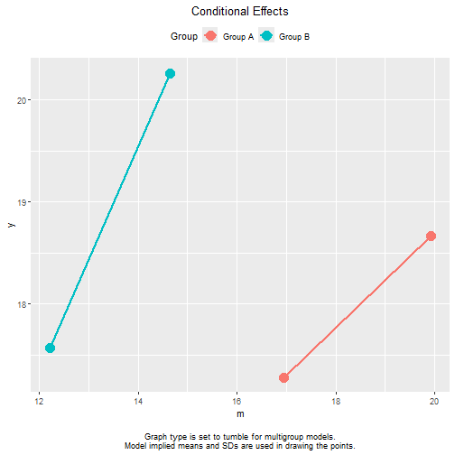
Note that, for multigroup models, the tumble graph proposed
by Bodner (2016) will always be used. The
position of a line for a group is determined by the model implied means
and SDs of this group. If no equality constraints imposed, these means
and SDs are close to the sample means and SDs. For example, the line
segment of "Group A" is far to the right because
"Group A" has a larger mean of m than
"Group B".
These are the model implied means and SDs:
# Model implied means
lavInspect(fit, "mean.ov")
#> $`Group A`
#>      m      y      x     c1     c2
#> 18.434 17.973  9.985  2.055  4.883
#>
#> $`Group B`
#>      m      y      x     c1     c2
#> 13.423 18.915 10.046  2.138  5.088

# Model implied SDs
tmp <- lavInspect(fit, "cov.ov")
sqrt(diag(tmp[["Group A"]]))
#>         m         y         x        c1        c2
#> 1.4916076 2.2158085 1.1055723 0.9687943 1.0741628
sqrt(diag(tmp[["Group B"]]))
#>         m         y         x        c1        c2
#> 1.2142143 2.5838604 1.0094330 0.9518064 1.0594076
It would be misleading if the two lines are plotted on the same
horizontal position, assuming incorrectly that the ranges of
m are similar in the two groups.
The vertical positions of the two lines are similarly determined by
the distributions of other predictors in each group (the control
variables and x in this example).
Details of the plot method can be found in the help
page.
Final Remarks
There are some limitations on the support for multigroup models.
Currently, multiple imputation is not supported. Moreover, most
functions do not (yet) support multigroup models with within-group
moderators, except for cond_indirect(). We would appreciate
users to report issues discovered when using manymome on
multigroup models at GitHub.