Moderated Mediation Analysis by Multiple Regression

Introduction

This article is a brief illustration of how to use cond_indirect_effects() from the package manymome (Cheung & Cheung, 2023) to estimate the conditional indirect effects when the model parameters are estimate by ordinary least squares (OLS) multiple regression using lm().

Data Set and Model

This is the sample data set used for illustration:

library(manymome)
dat <- data_med_mod_a
print(head(dat), digits = 3)
#>       x    w    m    y   c1   c2
#> 1  8.58 1.57 28.9 36.9 6.03 4.82
#> 2 10.36 1.10 24.8 24.5 5.19 5.34
#> 3 10.38 2.88 37.3 38.1 4.63 5.02
#> 4  9.53 3.16 32.6 37.9 2.94 6.01
#> 5 11.34 3.84 49.2 59.0 6.12 5.05
#> 6  9.66 2.22 26.4 35.4 4.02 5.03

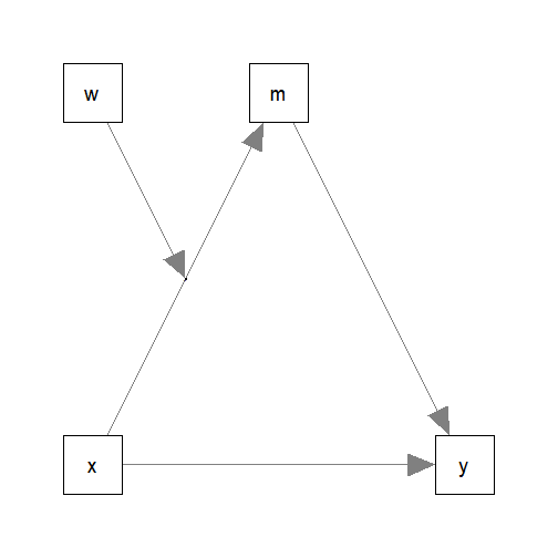
This dataset has 6 variables: one predictor (x), one mediators (m), one outcome variable (y), one moderator (w) and two control variables (c1 and c2).

Suppose this is the model being fitted:

plot of chunk mome_lm_draw_model

The path parameters can be estimated by two multiple regression models:

lm_m <- lm(m ~ x*w + c1 + c2, dat)
lm_y <- lm(y ~ m + x + c1 + c2, dat)

These are the estimates of the regression coefficient of the paths:

# ###### Predict m ######
#
summary(lm_m)
#> 
#> Call:
#> lm(formula = m ~ x * w + c1 + c2, data = dat)
#> 
#> Residuals:
#>     Min      1Q  Median      3Q     Max 
#> -8.5621 -2.0065 -0.2142  1.7618 10.4270 
#> 
#> Coefficients:
#>             Estimate Std. Error t value Pr(>|t|)  
#> (Intercept)  16.4910    12.1039   1.362   0.1763  
#> x             0.0959     1.1958   0.080   0.9362  
#> w            -3.4871     4.7907  -0.728   0.4685  
#> c1            0.5372     0.4162   1.291   0.2000  
#> c2           -0.1533     0.4211  -0.364   0.7165  
#> x:w           0.9785     0.4794   2.041   0.0441 *
#> ---
#> Signif. codes:  0 '***' 0.001 '**' 0.01 '*' 0.05 '.' 0.1 ' ' 1
#> 
#> Residual standard error: 3.998 on 94 degrees of freedom
#> Multiple R-squared:  0.7479, Adjusted R-squared:  0.7345 
#> F-statistic: 55.79 on 5 and 94 DF,  p-value: < 2.2e-16
#
# ###### Predict y ######
#
summary(lm_y)
#> 
#> Call:
#> lm(formula = y ~ m + x + c1 + c2, data = dat)
#> 
#> Residuals:
#>     Min      1Q  Median      3Q     Max 
#> -9.4396 -2.8156 -0.3145  2.3231 11.2849 
#> 
#> Coefficients:
#>             Estimate Std. Error t value Pr(>|t|)    
#> (Intercept)  4.50635    5.40625   0.834    0.407    
#> m            0.95867    0.05806  16.512   <2e-16 ***
#> x           -0.01980    0.50578  -0.039    0.969    
#> c1           0.68241    0.44110   1.547    0.125    
#> c2          -0.49573    0.44565  -1.112    0.269    
#> ---
#> Signif. codes:  0 '***' 0.001 '**' 0.01 '*' 0.05 '.' 0.1 ' ' 1
#> 
#> Residual standard error: 4.229 on 95 degrees of freedom
#> Multiple R-squared:  0.7669, Adjusted R-squared:  0.7571 
#> F-statistic: 78.15 on 4 and 95 DF,  p-value: < 2.2e-16

Although not mandatory, it is recommended to combine the models into one object (a system of regression models) using lm2list():

fit_lm <- lm2list(lm_m, lm_y)
fit_lm
#> 
#> The model(s):
#> m ~ x * w + c1 + c2
#> y ~ m + x + c1 + c2

Simply use the lm() outputs as arguments. Order does not matter. To ensure that the regression outputs can be validly combined, lm2list() will also check:

whether the same sample is used in all regression analysis (not just same sample size, but the same set of cases), and
whether the models are “connected”, to ensure that the regression outputs can be validly combined.

Generating Bootstrap Estimates

To form nonparametric bootstrap confidence interval for effects to be computed, do_boot() can be used to generate bootstrap estimates for all regression coefficients first. These estimates can be reused for any effects to be estimated.

boot_out_lm <- do_boot(fit_lm,
                       R = 100,
                       seed = 54532,
                       ncores = 1)

Please see vignette("do_boot") or the help page of do_boot() on how to use this function. In real research, R, the number of bootstrap samples, should be set to 2000 or even 5000. The argument ncores can usually be omitted unless users want to manually control the number of CPU cores used in parallel processing.

Conditional Indirect Effects

We can now use cond_indirect_effects() to estimate the indirect effects for different levels of the moderator (w) and form their bootstrap confidence interval. By reusing the generated bootstrap estimates, there is no need to repeat the resampling.

Suppose we want to estimate the indirect effect from x to y through m, conditional on w:

(Refer to vignette("manymome") and the help page of cond_indirect_effects() on the arguments.)

out_xmy_on_w <- cond_indirect_effects(wlevels = "w",
                                      x = "x",
                                      y = "y",
                                      m = "m",
                                      fit = fit_lm,
                                      boot_ci = TRUE,
                                      boot_out = boot_out_lm)
out_xmy_on_w
#> 
#> == Conditional indirect effects ==
#> 
#>  Path: x -> m -> y
#>  Conditional on moderator(s): w
#>  Moderator(s) represented by: w
#> 
#>       [w]   (w)   ind  CI.lo CI.hi Sig   m~x   y~m
#> 1 M+1.0SD 3.164 3.060  2.168 4.039 Sig 3.192 0.959
#> 2 Mean    2.179 2.136  1.407 2.925 Sig 2.228 0.959
#> 3 M-1.0SD 1.194 1.212 -0.288 2.564     1.265 0.959
#> 
#>  - [CI.lo to CI.hi] are 95.0% percentile confidence intervals by
#>    nonparametric bootstrapping with 100 samples.
#>  - The 'ind' column shows the conditional indirect effects.
#>  - 'm~x','y~m' is/are the path coefficient(s) along the path conditional
#>    on the moderator(s).

When w is one standard deviation below mean, the indirect effect is 1.212, with 95% confidence interval [-0.288, 2.564].

When w is one standard deviation above mean, the indirect effect is 3.060, with 95% confidence interval [2.168, 4.039].

Note that any conditional indirect path in the model can be estimated this way. There is no limit on the path to be estimated, as long as all required path coefficients are in the model. cond_indirect_effects() will also check whether a path is valid. However, for complicated models, structural equation modelling may be a more flexible approach than multiple regression.

Not covered here, but the index of moderated moderated mediation can also be estimated in models with two moderators on the same path, estimated by regression. See vignette("manymome") for an example.

Index of Moderated Mediation

The function index_of_mome() can be used to compute the index of moderated mediation of w on the path x -> m -> y:

(Refer to vignette("manymome") and the help page of index_of_mome() on the arguments.)

out_mome <- index_of_mome(x = "x",
                          y = "y",
                          m = "m",
                          w = "w",
                          fit = fit_lm,
                          boot_ci = TRUE,
                          boot_out = boot_out_lm)
out_mome
#> 
#> == Conditional indirect effects ==
#> 
#>  Path: x -> m -> y
#>  Conditional on moderator(s): w
#>  Moderator(s) represented by: w
#> 
#>   [w] (w)   ind  CI.lo CI.hi Sig   m~x   y~m
#> 1   1   1 1.030 -0.622 2.543     1.074 0.959
#> 2   0   0 0.092 -2.389 2.434     0.096 0.959
#> 
#> == Index of Moderated Mediation ==
#> 
#> Levels compared: Row 1 - Row 2
#> 
#>       x y Index CI.lo CI.hi
#> Index x y 0.938 0.178 1.732
#> 
#>  - [CI.lo, CI.hi]: 95% percentile confidence interval.

In this model, the index of moderated mediation is 0.938, with 95% bootstrap confidence interval [0.178, 1.732]. The indirect effect of x on y through m significantly changes when w increases by one unit.

Standardized Conditional Indirect effects

The standardized conditional indirect effect from x to y through m conditional on w can be estimated by setting standardized_x and standardized_y to TRUE:

std_xmy_on_w <- cond_indirect_effects(wlevels = "w",
                                      x = "x",
                                      y = "y",
                                      m = "m",
                                      fit = fit_lm,
                                      boot_ci = TRUE,
                                      boot_out = boot_out_lm,
                                      standardized_x = TRUE,
                                      standardized_y = TRUE)
std_xmy_on_w
#> 
#> == Conditional indirect effects ==
#> 
#>  Path: x -> m -> y
#>  Conditional on moderator(s): w
#>  Moderator(s) represented by: w
#> 
#>       [w]   (w)   std  CI.lo CI.hi Sig   m~x   y~m   ind
#> 1 M+1.0SD 3.164 0.318  0.220 0.437 Sig 3.192 0.959 3.060
#> 2 Mean    2.179 0.222  0.134 0.309 Sig 2.228 0.959 2.136
#> 3 M-1.0SD 1.194 0.126 -0.031 0.260     1.265 0.959 1.212
#> 
#>  - [CI.lo to CI.hi] are 95.0% percentile confidence intervals by
#>    nonparametric bootstrapping with 100 samples.
#>  - std: The standardized conditional indirect effects. 
#>  - ind: The unstandardized conditional indirect effects.
#>  - 'm~x','y~m' is/are the path coefficient(s) along the path conditional
#>    on the moderator(s).

The standardized indirect effect is 0.126, with 95% confidence interval [-0.031, 0.260].

More Complicated Models

After the regression coefficients are estimated, cond_indirect_effects(), indirect_effect(), and related functions are used in the same way as for models fitted by lavaan::sem(). The levels for the moderators are controlled by mod_levels() and related functions in the same way whether a model is fitted by lavaan::sem() or lm(). Pplease refer to other articles (e.g., vignette("manymome") and vignette("mod_levels")) on how to estimate effects in other model analyzed by multiple regression.

Reference

Cheung, S. F., & Cheung, S.-H. (2023). manymome: An R package for computing the indirect effects, conditional effects, and conditional indirect effects, standardized or unstandardized, and their bootstrap confidence intervals, in many (though not all) models. Behavior Research Methods. https://doi.org/10.3758/s13428-023-02224-z

Shu Fai Cheung & Sing-Hang Cheung

2024-10-04