Moderated Regression: Categorical Moderators

Introduction

This article is part of a series of brief illustrations of how to use cond_effects() from the package manymome (Cheung & Cheung, 2024) to estimate the conditional effects when the model parameters are estimate by ordinary least squares (OLS) multiple regression using lm(). For moderated mediation tested by OLS regression, please refer to this article.

(Articles in this series had duplicated sections, to make each of them self-contained.)

Data Set and Model

This is the sample data set used for illustration:

library(manymome)
dat <- data_mod_cat_2w
print(head(dat), digits = 3)
#>      x    y   c1   c2      gp   site
#> 1 19.8 24.5 29.5 10.2 Control Site 1
#> 2 24.0 21.6 15.3 10.3 Control Site 1
#> 3 28.4 24.7 29.4 20.4 Control Site 1
#> 4 39.7 26.9 32.4 16.7 Control Site 1
#> 5 33.4 21.1 36.5 10.2 Control Site 1
#> 6 22.7 23.8 27.9 23.5 Control Site 1

This dataset has 6 variables:

one outcome variable (y),
one predictor (x),
two categorical moderators (gp, site),
two control variables (c1 and c2).

The moderator gp has two possible values: "Control" and "Treatment".

The moderator site has three possible values: "Site 1", "Site 2", and "Site 3".

We will first consider two models, each with only one of the two moderators.

One Categorical Moderator: Two Categories

Suppose this is the model being fitted, with control variables omitted from the plot for readability:

Model: gp

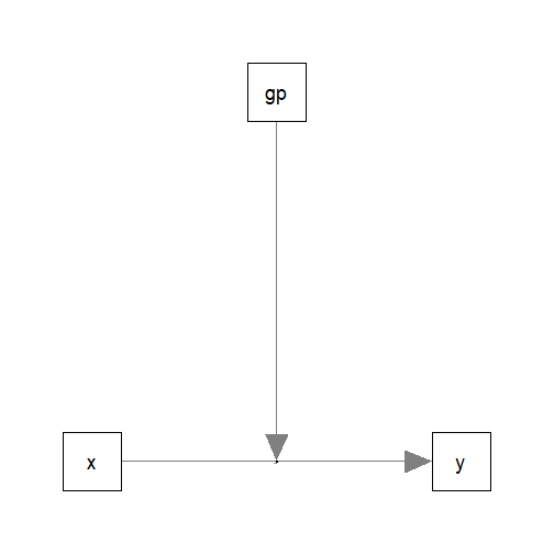
Fit by Regression

The path parameters can be estimated by multiple regression using lm():

lm_y_gp <- lm(
  y ~ gp*x + c1 + c2,
  data = dat
)

These are the estimates of the regression coefficient of the paths:

summary(lm_y_gp)
#> 
#> Call:
#> lm(formula = y ~ gp * x + c1 + c2, data = dat)
#> 
#> Residuals:
#>      Min       1Q   Median       3Q      Max 
#> -10.8400  -2.6594  -0.2263   2.6201  15.5956 
#> 
#> Coefficients:
#>               Estimate Std. Error t value Pr(>|t|)    
#> (Intercept)   20.26140    1.49550  13.548  < 2e-16 ***
#> gpTreatment   -4.96460    1.09316  -4.542 6.77e-06 ***
#> x             -0.02738    0.03674  -0.745    0.456    
#> c1            -0.02833    0.03843  -0.737    0.461    
#> c2             0.39637    0.04438   8.932  < 2e-16 ***
#> gpTreatment:x  0.34746    0.04953   7.015 6.31e-12 ***
#> ---
#> Signif. codes:  0 '***' 0.001 '**' 0.01 '*' 0.05 '.' 0.1 ' ' 1
#> 
#> Residual standard error: 4.093 on 594 degrees of freedom
#> Multiple R-squared:  0.2698, Adjusted R-squared:  0.2636 
#> F-statistic: 43.89 on 5 and 594 DF,  p-value: < 2.2e-16

Conditional Effects

We can now use cond_effects() to estimate the effects of x on y for different categories of the moderator gp.

(Refer to vignette("manymome") and the help page of cond_effects() on the arguments.)

out_gp <- cond_effects(
  wlevels = "gp",
  x = "x",
  y = "y",
  fit = lm_y_gp
)
out_gp
#> 
#> == Conditional effects ==
#> 
#>  Path: x -> y
#>  Conditional on moderator(s): gp
#>  Moderator(s) represented by: gpTreatment
#> 
#>        [gp] (gpTreatment)    ind    SE   Stat pvalue Sig  CI.lo CI.hi
#> 1 Control               0 -0.027 0.037 -0.745  0.456     -0.100 0.045
#> 2 Treatment             1  0.320 0.033  9.655  0.000 ***  0.255 0.385
#> 
#>  - [SE] are regression standard errors.
#>  - [Stat] are the t statistics used to test the effects.
#>  - [pvalue] are p-values computed from 'Stat'.
#>  - [Sig]: 0 '***' 0.001 '**' 0.01 '*' 0.05 ' ' 1.
#>  - [CI.lo to CI.hi] are 95.0% confidence interval computed from regression standard errors.
#>  - The 'ind' column shows the conditional effects.
#>

The column ind show the effects of x on y for different categories of gp.

In the group "Control", the effect of x is -0.027, with 95% confidence interval [-0.100, 0.045].

In the group "Treatment", the effect of x is 0.320, with 95% confidence interval [0.255, 0.385].

NOTE: The standard error (SE) and related results are computed using the pick-a-point approach by Rogosa (1980).

Plotting the Conditional Effects

The output of cond_effects() has a plot method for plotting the conditional effects:

plot(out_gp)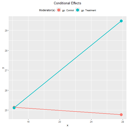

Conventional Plot of Conditional Effects (gp)

By default, the lines span the range of one standard deviation below and above the mean of the predictor.

The plot can be customized in a lot of way. Please refer to the help page of plot.cond_indirect_effects() for available options.

Tumble Plot

If the distribution of the x variable may vary for different levels of the moderators, a version of tumble graph proposed by Bodner (2016) can be plotted by adding graph_type = "tumble":

plot(out_gp,
     graph_type = "tumble")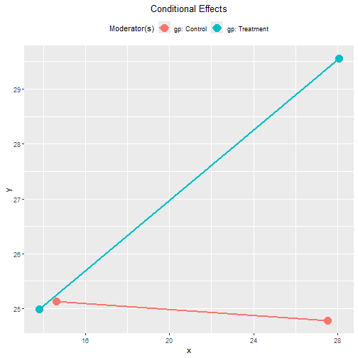

Tumble Plot of Conditional Effects (gp)

In this example, the distributions of x for the groups are similar.

Standardized Conditional Effects

Although OLS can be used to estimate and test the unstandardized effects, it is inappropriate for forming the confidence intervals for the standardized effects. See Yuan & Chan (2011) on the issue on standardized regression coefficients.

To form nonparametric bootstrap confidence interval for effects to be computed, add boot_ci = TRUE, R to the number of bootstrap samples (should be 5000 or even 10000, for multiple regression), and seed (set it to an integer to ensure the results are reproducible).

The standardized conditional effects from x to y conditional on gp can be estimated by setting standardized_x and standardized_y to TRUE.

This is the output:

std_gp <- cond_effects(
  wlevels = "gp",
  x = "x",
  y = "y",
  fit = lm_y_gp,
  boot_ci = TRUE,
  R = 5000,
  seed = 54532,
  standardized_x = TRUE,
  standardized_y = TRUE
)
#> 19 processes started to run bootstrapping.
std_gp
#> 
#> == Conditional effects ==
#> 
#>  Path: x -> y
#>  Conditional on moderator(s): gp
#>  Moderator(s) represented by: gpTreatment
#> 
#>        [gp] (gpTreatment)    std  CI.lo CI.hi Sig    ind
#> 1 Control               0 -0.039 -0.130 0.048     -0.027
#> 2 Treatment             1  0.457  0.363 0.551 Sig  0.320
#> 
#>  - [CI.lo to CI.hi] are 95.0% percentile confidence intervals by nonparametric bootstrapping with 5000
#>    samples.
#>  - std: The standardized conditional effects. 
#>  - ind: The unstandardized conditional effects.
#>

In the group "Control", the standardized effect of x is -0.039, with 95% confidence interval [-0.130, 0.048].

In the group "Treatment", the standardized effect of x is 0.457, with 95% confidence interval [0.363, 0.551].

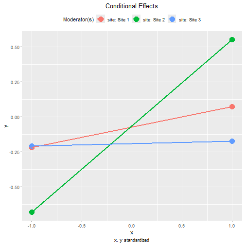
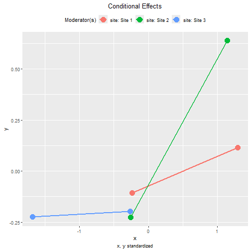
Plot Standardized Conditional Effects

The plot() method can also be used on the standardized conditional effects, although the only differences are the values displayed on the axes:

plot(std_gp)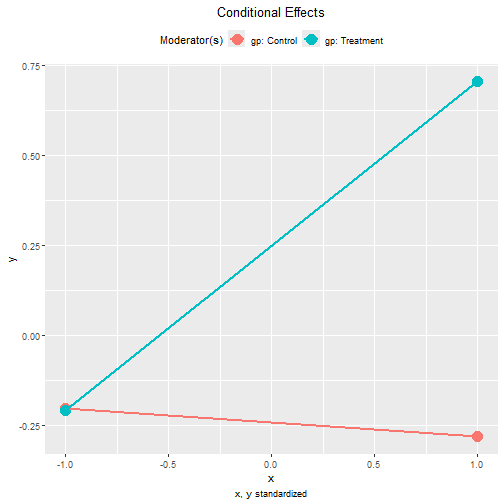

Conventional Plot of Standardized Conditional Effects (gp)

plot(std_gp,
     graph_type = "tumble")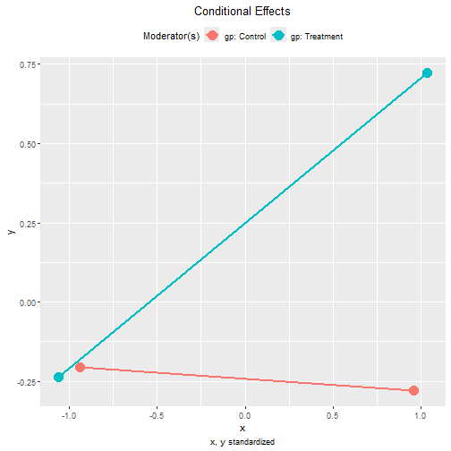

Tumble Plot of Standardized Conditional Effects (gp)

One Categorical Moderator: Three Categories

The steps demonstrated above can be used for a categorical moderator with any number of levels.

Suppose this is the model being fitted, with control variables omitted from the plot for readability:

Model: site

Fit by Regression

The path parameters can be estimated by a multiple regression model:

lm_y_site <- lm(
  y ~ site*x + c1 + c2,
  data = dat
)

These are the estimates of the regression coefficient of the paths:

summary(lm_y_site)
#> 
#> Call:
#> lm(formula = y ~ site * x + c1 + c2, data = dat)
#> 
#> Residuals:
#>      Min       1Q   Median       3Q      Max 
#> -12.2398  -3.0852   0.2666   2.7867  17.3110 
#> 
#> Coefficients:
#>              Estimate Std. Error t value Pr(>|t|)    
#> (Intercept)  19.01557    1.99047   9.553  < 2e-16 ***
#> siteSite 2   -6.89570    2.15974  -3.193 0.001484 ** 
#> siteSite 3    1.30350    1.76713   0.738 0.461027    
#> x             0.10205    0.05877   1.737 0.082989 .  
#> c1           -0.03133    0.04062  -0.771 0.440934    
#> c2            0.35831    0.04681   7.655 7.91e-14 ***
#> siteSite 2:x  0.32975    0.08710   3.786 0.000169 ***
#> siteSite 3:x -0.08913    0.08673  -1.028 0.304478    
#> ---
#> Signif. codes:  0 '***' 0.001 '**' 0.01 '*' 0.05 '.' 0.1 ' ' 1
#> 
#> Residual standard error: 4.317 on 592 degrees of freedom
#> Multiple R-squared:  0.1905, Adjusted R-squared:  0.1809 
#> F-statistic:  19.9 on 7 and 592 DF,  p-value: < 2.2e-16

Conditional Effects

The function cond_effects() will determine the number of categories automatically:

out_site <- cond_effects(
  wlevels = "site",
  x = "x",
  y = "y",
  fit = lm_y_site
)
out_site
#> 
#> == Conditional effects ==
#> 
#>  Path: x -> y
#>  Conditional on moderator(s): site
#>  Moderator(s) represented by: siteSite 2, siteSite 3
#> 
#>   [site] (siteSite 2) (siteSite 3)   ind    SE  Stat pvalue Sig  CI.lo CI.hi
#> 1 Site 1            0            0 0.102 0.059 1.737  0.083     -0.013 0.217
#> 2 Site 2            1            0 0.432 0.064 6.715  0.000 ***  0.306 0.558
#> 3 Site 3            0            1 0.013 0.064 0.203  0.840     -0.112 0.138
#> 
#>  - [SE] are regression standard errors.
#>  - [Stat] are the t statistics used to test the effects.
#>  - [pvalue] are p-values computed from 'Stat'.
#>  - [Sig]: 0 '***' 0.001 '**' 0.01 '*' 0.05 ' ' 1.
#>  - [CI.lo to CI.hi] are 95.0% confidence interval computed from regression standard errors.
#>  - The 'ind' column shows the conditional effects.
#>

In the site "Site 1", the effect of x is 0.102, with 95% confidence interval [-0.013, 0.217].

In the site "Site 2", the effect of x is 0.432, with 95% confidence interval [0.306, 0.558].

In the site "Site 3", the effect of x is 0.013, with 95% confidence interval [-0.112, 0.138].

Plotting the Conditional Effects

These are the plots of the conditional effects:

plot(out_site)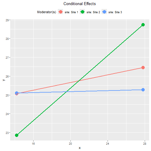

Conventional Plot of Conditional Effects (site)

plot(out_site,
     graph_type = "tumble")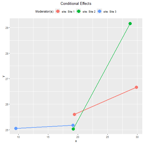

Tumble Plot of Conditional Effects (site)

This example demonstrates the advantage of the tumble graph. The distribution of x in "Site 3" has a mean lower than those in the other two sites. The conventional plot using the same range of x in all three groups will give the incorrect impression of a cross-over of the lines in the samples (though it is possible that such a cross-over of the lines happens in the populations).

Standardized Conditional Effects

This is the output of the standardized conditional effects, with bootstrap confidence intervals:

std_site <- cond_effects(
  wlevels = "site",
  x = "x",
  y = "y",
  fit = lm_y_site,
  boot_ci = TRUE,
  R = 5000,
  seed = 54532,
  standardized_x = TRUE,
  standardized_y = TRUE
)
#> 19 processes started to run bootstrapping.
std_site
#> 
#> == Conditional effects ==
#> 
#>  Path: x -> y
#>  Conditional on moderator(s): site
#>  Moderator(s) represented by: siteSite 2, siteSite 3
#> 
#>   [site] (siteSite 2) (siteSite 3)   std  CI.lo CI.hi Sig   ind
#> 1 Site 1            0            0 0.146 -0.023 0.317     0.102
#> 2 Site 2            1            0 0.616  0.414 0.818 Sig 0.432
#> 3 Site 3            0            1 0.018 -0.157 0.201     0.013
#> 
#>  - [CI.lo to CI.hi] are 95.0% percentile confidence intervals by nonparametric bootstrapping with 5000
#>    samples.
#>  - std: The standardized conditional effects. 
#>  - ind: The unstandardized conditional effects.
#>

Plot Standardized Conditional Effects

These are the plots of the standardized conditional effects:

plot(std_site)

Conventional Plot of Standardized Conditional Effects (site)

plot(std_site,
     graph_type = "tumble")

Tumble Plot of Standardized Conditional Effects (site)

Two Categorical Moderators

The steps demonstrated above can be used in a regression model with any number of moderators.

Suppose this is the model being fitted, with control variables omitted from the plot for readability, both gp and site included, but no interaction between them:

Model: gp + site

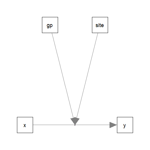
Fit by Regression

We first fit the regression model as usual:

lm_y_gp_site <- lm(
  y ~ gp*x + site*x + c1 + c2,
  data = dat
)

These are the estimates of the regression coefficient of the paths:

summary(lm_y_gp_site)
#> 
#> Call:
#> lm(formula = y ~ gp * x + site * x + c1 + c2, data = dat)
#> 
#> Residuals:
#>      Min       1Q   Median       3Q      Max 
#> -11.4604  -2.5856  -0.0874   2.5927  14.1720 
#> 
#> Coefficients:
#>               Estimate Std. Error t value Pr(>|t|)    
#> (Intercept)   21.09442    1.89659  11.122  < 2e-16 ***
#> gpTreatment   -5.24348    1.07451  -4.880 1.37e-06 ***
#> x             -0.08388    0.05955  -1.409 0.159472    
#> siteSite 2    -6.51680    2.00106  -3.257 0.001192 ** 
#> siteSite 3     1.39984    1.64547   0.851 0.395268    
#> c1            -0.01832    0.03766  -0.486 0.626860    
#> c2             0.38081    0.04345   8.764  < 2e-16 ***
#> gpTreatment:x  0.35510    0.04857   7.312 8.64e-13 ***
#> x:siteSite 2   0.31277    0.08070   3.876 0.000118 ***
#> x:siteSite 3  -0.08921    0.08091  -1.103 0.270626    
#> ---
#> Signif. codes:  0 '***' 0.001 '**' 0.01 '*' 0.05 '.' 0.1 ' ' 1
#> 
#> Residual standard error: 3.999 on 590 degrees of freedom
#> Multiple R-squared:  0.3077, Adjusted R-squared:  0.2971 
#> F-statistic: 29.13 on 9 and 590 DF,  p-value: < 2.2e-16

Conditional Effects

The function cond_effects() can be used for any number of moderators, as long as they are listed in wlevels:

out_gp_site <- cond_effects(
  wlevels = c("gp", "site"),
  x = "x",
  y = "y",
  fit = lm_y_gp_site
)
out_gp_site
#> 
#> == Conditional effects ==
#> 
#>  Path: x -> y
#>  Conditional on moderator(s): gp, site
#>  Moderator(s) represented by: gpTreatment, siteSite 2, siteSite 3
#> 
#>        [gp] [site] (gpTreatment) (siteSite 2) (siteSite 3)    ind    SE   Stat pvalue Sig  CI.lo  CI.hi
#> 1 Control   Site 1             0            0            0 -0.084 0.060 -1.409  0.159     -0.201  0.033
#> 2 Control   Site 2             0            1            0  0.229 0.065  3.527  0.000 ***  0.101  0.356
#> 3 Control   Site 3             0            0            1 -0.173 0.067 -2.592  0.010 **  -0.304 -0.042
#> 4 Treatment Site 1             1            0            0  0.271 0.060  4.543  0.000 ***  0.154  0.388
#> 5 Treatment Site 2             1            1            0  0.584 0.064  9.146  0.000 ***  0.459  0.709
#> 6 Treatment Site 3             1            0            1  0.182 0.062  2.936  0.003 **   0.060  0.304
#> 
#>  - [SE] are regression standard errors.
#>  - [Stat] are the t statistics used to test the effects.
#>  - [pvalue] are p-values computed from 'Stat'.
#>  - [Sig]: 0 '***' 0.001 '**' 0.01 '*' 0.05 ' ' 1.
#>  - [CI.lo to CI.hi] are 95.0% confidence interval computed from regression standard errors.
#>  - The 'ind' column shows the conditional effects.
#>

IMPORTANT: Even though this model does not have three-way interaction, the conditional effects still need to consider both moderators. It is because the effect of x depends on all moderators, whether there is higher order interaction or not.

If one or more moderators are omitted, a warning message will be issued. This is an example:

cond_effects(
  wlevels = "gp",
  x = "x",
  y = "y",
  fit = lm_y_gp_site
)
#> Warning in (function (xi, yi, yiname, digits = 3, y, wvalues = NULL, warn = TRUE, : siteSite 2, siteSite 3 modelled as
#> moderator(s) for the path from y~x to y but not included in 'wvalues'. They will be set to zero in computing the
#> conditional effect, which may not be meaningful. Please check.
#> Warning in (function (xi, yi, yiname, digits = 3, y, wvalues = NULL, warn = TRUE, : siteSite 2, siteSite 3 modelled as
#> moderator(s) for the path from y~x to y but not included in 'wvalues'. They will be set to zero in computing the
#> conditional effect, which may not be meaningful. Please check.
#> 
#> == Conditional effects ==
#> 
#>  Path: x -> y
#>  Conditional on moderator(s): gp
#>  Moderator(s) represented by: gpTreatment
#> 
#>        [gp] (gpTreatment)    ind    SE   Stat pvalue Sig  CI.lo CI.hi
#> 1 Control               0 -0.084 0.060 -1.409  0.159     -0.201 0.033
#> 2 Treatment             1  0.271 0.060  4.543  0.000 ***  0.154 0.388
#> 
#>  - [SE] are regression standard errors.
#>  - [Stat] are the t statistics used to test the effects.
#>  - [pvalue] are p-values computed from 'Stat'.
#>  - [Sig]: 0 '***' 0.001 '**' 0.01 '*' 0.05 ' ' 1.
#>  - [CI.lo to CI.hi] are 95.0% confidence interval computed from regression standard errors.
#>  - The 'ind' column shows the conditional effects.
#>

Plotting the Conditional Effects

Conventional Plots

These are the plots of the conditional effects:

plot(out_gp_site)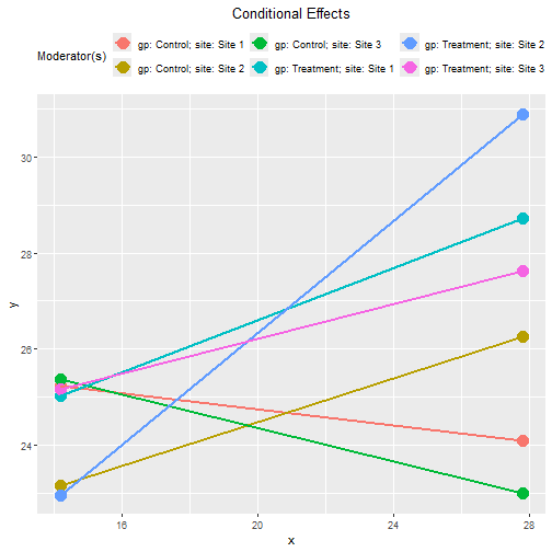

Conventional Plot of Conditional Effects (gp + site)

For two or more moderators, it is not easy to visualize the conditional effects if all lines are plotted on the same graph.

The argument facet_grid_cols can be used to plot the effect of one moderator for each category of the other moderator.

This is the plot of effects for "Control" and "Treatment":

plot(out_gp_site,
     facet_grid_cols = "gp")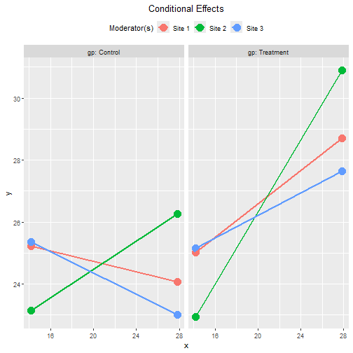

Conventional Plot of Conditional Effects: Site within Group

This is the plot of effects for each site:

plot(out_gp_site,
     facet_grid_cols = "site")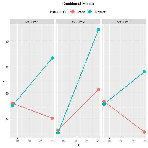

Conventional Plot of Conditional Effects: Group within Site

Note that, without three-way interaction, the moderating effect of gp is the same in all three sites, and the moderating effect of site is the same in all two groups. The six lines are different simply because the effect of x depends on both gp and site. They do not denote three-way interaction (because it is not in the regression model).

Tumble Plots

We already know the distributions of x are not the same in all three sites. Therefore, the tumble graph is a better way to visualize the effects:

plot(out_gp_site,
     facet_grid_cols = "gp",
     graph_type = "tumble")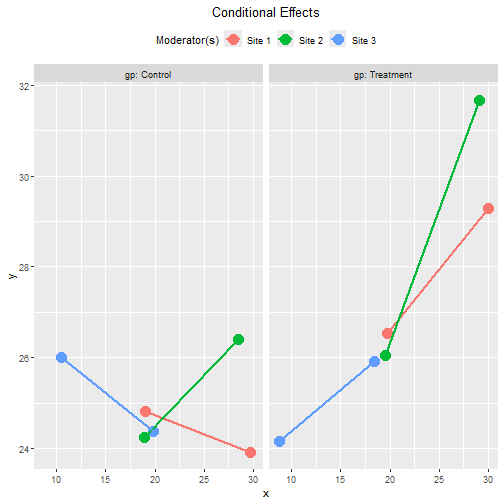

Tumble Plot of Conditional Effects: Group within Site

plot(out_gp_site,
     facet_grid_cols = "site",
     graph_type = "tumble")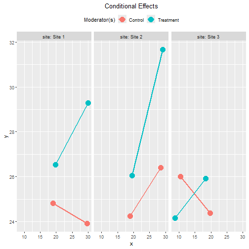

Tumble Plot of Conditional Effects: Site within Group

Standardized Conditional Effects

This is the output of the standardized conditional effects, with bootstrap confidence intervals:

std_gp_site <- cond_effects(
  wlevels = c("gp", "site"),
  x = "x",
  y = "y",
  fit = lm_y_gp_site,
  boot_ci = TRUE,
  R = 5000,
  seed = 54532,
  standardized_x = TRUE,
  standardized_y = TRUE
)
#> 19 processes started to run bootstrapping.
std_gp_site
#> 
#> == Conditional effects ==
#> 
#>  Path: x -> y
#>  Conditional on moderator(s): gp, site
#>  Moderator(s) represented by: gpTreatment, siteSite 2, siteSite 3
#> 
#>        [gp] [site] (gpTreatment) (siteSite 2) (siteSite 3)    std  CI.lo  CI.hi Sig    ind
#> 1 Control   Site 1             0            0            0 -0.120 -0.275  0.035     -0.084
#> 2 Control   Site 2             0            1            0  0.327  0.153  0.495 Sig  0.229
#> 3 Control   Site 3             0            0            1 -0.247 -0.460 -0.027 Sig -0.173
#> 4 Treatment Site 1             1            0            0  0.387  0.220  0.549 Sig  0.271
#> 5 Treatment Site 2             1            1            0  0.833  0.650  1.009 Sig  0.584
#> 6 Treatment Site 3             1            0            1  0.260  0.068  0.466 Sig  0.182
#> 
#>  - [CI.lo to CI.hi] are 95.0% percentile confidence intervals by nonparametric bootstrapping with 5000
#>    samples.
#>  - std: The standardized conditional effects. 
#>  - ind: The unstandardized conditional effects.
#>

Tumble Plots of Standardized Conditional Effects

These are the plots of the standardized conditional effects, with facet_grid_cols set:

plot(std_gp_site,
     facet_grid_cols = "gp",
     graph_type = "tumble")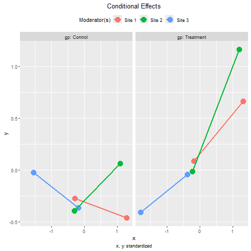

Tumble Plot of Standardized Conditional Effects: Site within Group

plot(std_gp_site,
     facet_grid_cols = "site",
     graph_type = "tumble")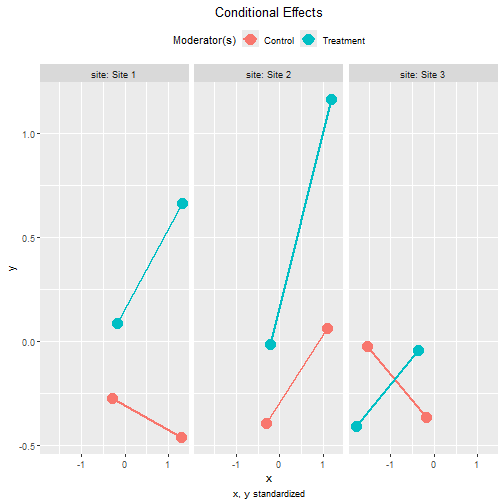

Tumble Plot of Standardized Conditional Effects: Group within Site

Two Categorical Moderators, with Three-Way Interaction

Suppose that we suspect that the two categorical moderators interact with each other. That is, the group difference in the effect of x may not be the same in all three sites, or the site difference in the effect of x may not be the same in the two groups.

The steps demonstrated above can also be used in this regression model:

lm_y_gp_x_site <- lm(
  y ~ x*site*gp + c1 + c2,
  data = dat
)

The test of the difference between this model and the previous model with no three-way interaction supports that this model fits better:

anova(
  lm_y_gp_site,
  lm_y_gp_x_site
)
#> Analysis of Variance Table
#> 
#> Model 1: y ~ gp * x + site * x + c1 + c2
#> Model 2: y ~ x * site * gp + c1 + c2
#>   Res.Df    RSS Df Sum of Sq      F    Pr(>F)    
#> 1    590 9436.6                                  
#> 2    586 9108.5  4    328.07 5.2766 0.0003516 ***
#> ---
#> Signif. codes:  0 '***' 0.001 '**' 0.01 '*' 0.05 '.' 0.1 ' ' 1

These are the estimates of the regression coefficient of this model:

summary(lm_y_gp_x_site)
#> 
#> Call:
#> lm(formula = y ~ x * site * gp + c1 + c2, data = dat)
#> 
#> Residuals:
#>      Min       1Q   Median       3Q      Max 
#> -11.0954  -2.5367  -0.0151   2.4875  14.3118 
#> 
#> Coefficients:
#>                           Estimate Std. Error t value Pr(>|t|)    
#> (Intercept)              22.077128   2.213474   9.974  < 2e-16 ***
#> x                        -0.128074   0.074369  -1.722  0.08557 .  
#> siteSite 2               -5.276352   2.748471  -1.920  0.05538 .  
#> siteSite 3               -3.063916   2.296016  -1.334  0.18258    
#> gpTreatment              -8.501074   2.708983  -3.138  0.00179 ** 
#> c1                       -0.002987   0.037316  -0.080  0.93622    
#> c2                        0.385877   0.042952   8.984  < 2e-16 ***
#> x:siteSite 2              0.222148   0.112091   1.982  0.04796 *  
#> x:siteSite 3              0.154193   0.113159   1.363  0.17352    
#> x:gpTreatment             0.453702   0.107574   4.218 2.86e-05 ***
#> siteSite 2:gpTreatment   -1.970235   3.954140  -0.498  0.61848    
#> siteSite 3:gpTreatment    8.743721   3.254470   2.687  0.00742 ** 
#> x:siteSite 2:gpTreatment  0.157510   0.159449   0.988  0.32364    
#> x:siteSite 3:gpTreatment -0.485461   0.160220  -3.030  0.00255 ** 
#> ---
#> Signif. codes:  0 '***' 0.001 '**' 0.01 '*' 0.05 '.' 0.1 ' ' 1
#> 
#> Residual standard error: 3.943 on 586 degrees of freedom
#> Multiple R-squared:  0.3317, Adjusted R-squared:  0.3169 
#> F-statistic: 22.38 on 13 and 586 DF,  p-value: < 2.2e-16

Conditional Effects

The function cond_effects() can be used in exactly the same way, whether the moderators interact with each other or not:

out_gp_x_site <- cond_effects(
  wlevels = c("site", "gp"),
  x = "x",
  y = "y",
  fit = lm_y_gp_x_site
)
out_gp_x_site
#> 
#> == Conditional effects ==
#> 
#>  Path: x -> y
#>  Conditional on moderator(s): site, gp
#>  Moderator(s) represented by: siteSite 2, siteSite 3, gpTreatment
#> 
#>   [site]      [gp] (siteSite 2) (siteSite 3) (gpTreatment)    ind    SE   Stat pvalue Sig  CI.lo CI.hi
#> 1 Site 1 Control              0            0             0 -0.128 0.074 -1.722  0.086     -0.274 0.018
#> 2 Site 1 Treatment            0            0             1  0.326 0.078  4.190  0.000 ***  0.173 0.478
#> 3 Site 2 Control              1            0             0  0.094 0.084  1.122  0.262     -0.071 0.259
#> 4 Site 2 Treatment            1            0             1  0.705 0.083  8.543  0.000 ***  0.543 0.867
#> 5 Site 3 Control              0            1             0  0.026 0.085  0.307  0.759     -0.141 0.193
#> 6 Site 3 Treatment            0            1             1 -0.006 0.082 -0.069  0.945     -0.167 0.156
#> 
#>  - [SE] are regression standard errors.
#>  - [Stat] are the t statistics used to test the effects.
#>  - [pvalue] are p-values computed from 'Stat'.
#>  - [Sig]: 0 '***' 0.001 '**' 0.01 '*' 0.05 ' ' 1.
#>  - [CI.lo to CI.hi] are 95.0% confidence interval computed from regression standard errors.
#>  - The 'ind' column shows the conditional effects.
#>

Plotting the Conditional Effects

These are the tumble plots of the conditional effects, with facet_grid_cols set:

plot(out_gp_x_site,
     facet_grid_cols = "gp",
     graph_type = "tumble")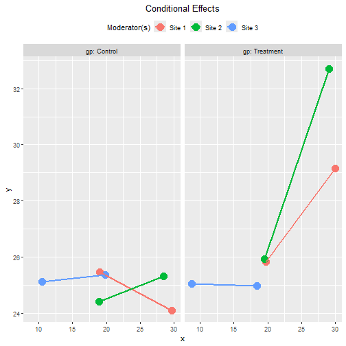

Tumble Plot of Conditional Effects: Site within Group

plot(out_gp_x_site,
     facet_grid_cols = "site",
     graph_type = "tumble")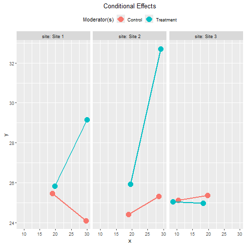

Tumble Plot of Conditional Effects: Group within Site

Standardized Conditional Effects

This is the output of the standardized conditional effects, with bootstrap confidence intervals:

std_gp_x_site <- cond_effects(
  wlevels = c("gp", "site"),
  x = "x",
  y = "y",
  fit = lm_y_gp_x_site,
  boot_ci = TRUE,
  R = 5000,
  seed = 54532,
  standardized_x = TRUE,
  standardized_y = TRUE
)
#> 19 processes started to run bootstrapping.
std_gp_x_site
#> 
#> == Conditional effects ==
#> 
#>  Path: x -> y
#>  Conditional on moderator(s): gp, site
#>  Moderator(s) represented by: gpTreatment, siteSite 2, siteSite 3
#> 
#>        [gp] [site] (gpTreatment) (siteSite 2) (siteSite 3)    std  CI.lo CI.hi Sig    ind
#> 1 Control   Site 1             0            0            0 -0.183 -0.374 0.003     -0.128
#> 2 Control   Site 2             0            1            0  0.134 -0.045 0.298      0.094
#> 3 Control   Site 3             0            0            1  0.037 -0.252 0.316      0.026
#> 4 Treatment Site 1             1            0            0  0.465  0.226 0.692 Sig  0.326
#> 5 Treatment Site 2             1            1            0  1.006  0.740 1.269 Sig  0.705
#> 6 Treatment Site 3             1            0            1 -0.008 -0.229 0.231     -0.006
#> 
#>  - [CI.lo to CI.hi] are 95.0% percentile confidence intervals by nonparametric bootstrapping with 5000
#>    samples.
#>  - std: The standardized conditional effects. 
#>  - ind: The unstandardized conditional effects.
#>

These are the plots of the standardized conditional effects, with facet_grid_cols set:

plot(std_gp_x_site,
     facet_grid_cols = "gp",
     graph_type = "tumble")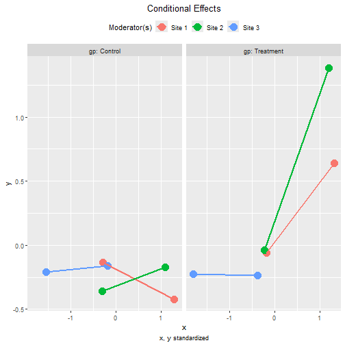

Tumble Plot of Standardized Conditional Effects: Site within Group

plot(std_gp_x_site,
     facet_grid_cols = "site",
     graph_type = "tumble")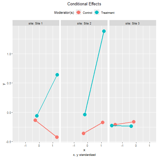

Tumble Plot of Standardized Conditional Effects: Group within Site

Other Moderated Regression Models

The function cond_effects() has no limit on the number of moderators and the number of predictors with their effects moderated.

The demonstrations of other moderated regression models can be found from the list of articles.

The levels for the moderators are controlled by mod_levels() and related functions in the same way whether a model is fitted by lavaan::sem() or lm(). Please refer to other articles (e.g., vignette("manymome") and vignette("mod_levels")) on how to estimate effects in other model analyzed by multiple regression.

References

Bodner, T. E. (2016). Tumble graphs: Avoiding misleading end point extrapolation when graphing interactions from a moderated multiple regression analysis. Journal of Educational and Behavioral Statistics, 41(6), 593–604. https://doi.org/10.3102/1076998616657080

Cheung, S. F., & Cheung, S.-H. (2024). Manymome: An R package for computing the indirect effects, conditional effects, and conditional indirect effects, standardized or unstandardized, and their bootstrap confidence intervals, in many (though not all) models. Behavior Research Methods, 56(5), 4862–4882. https://doi.org/10.3758/s13428-023-02224-z

Rogosa, D. (1980). Comparing nonparallel regression lines. Psychological Bulletin, 88(2), 307–321. https://doi.org/10.1037/0033-2909.88.2.307

Yuan, K.-H., & Chan, W. (2011). Biases and standard errors of standardized regression coefficients. Psychometrika, 76(4), 670–690. https://doi.org/10.1007/s11336-011-9224-6

Shu Fai Cheung & Sing-Hang Cheung

2026-07-03

Introduction

Data Set and Model

One Categorical Moderator: Two Categories

Fit by Regression

Conditional Effects

Plotting the Conditional Effects

Tumble Plot

Standardized Conditional Effects

Plot Standardized Conditional Effects

One Categorical Moderator: Three Categories

Fit by Regression

Conditional Effects

Plotting the Conditional Effects

Standardized Conditional Effects

Plot Standardized Conditional Effects

Two Categorical Moderators

Fit by Regression

Conditional Effects

Plotting the Conditional Effects

Conventional Plots

Tumble Plots

Standardized Conditional Effects

Tumble Plots of Standardized Conditional Effects

Two Categorical Moderators, with Three-Way Interaction

Conditional Effects

Plotting the Conditional Effects

Standardized Conditional Effects

Other Moderated Regression Models

References