Quick Function: Parallel Mediation with Observed Variables
2026-03-07
Source:vignettes/articles/template_q_med_obs_parallel.Rmd
template_q_med_obs_parallel.RmdIntroduction
This and other “Quick Function” articles are examples of R code to:
estimate the power,
search for a sample size with a target level of power, or
determine the range of sample sizes for a target level of power
for a specific scenario in typical mediation models using power4mome.
Users can quickly adapt them for their scenarios. They are how-to guides
and will not cover the technical details involved.
Prerequisite
These functions are wrappers to power4test(),
n_from_power(), and n_region_from_power(). For
simple scenarios, users do not need to know how to use these advanced
functions, though knowledge about them can help customizing the search
for the region. Further information on these functions can be found in
Final Remarks
Scope
This file is for parallel mediation models, and only use one function
q_power_mediation_parallel() from the package power4mome.
The Model
Suppose this is the model:
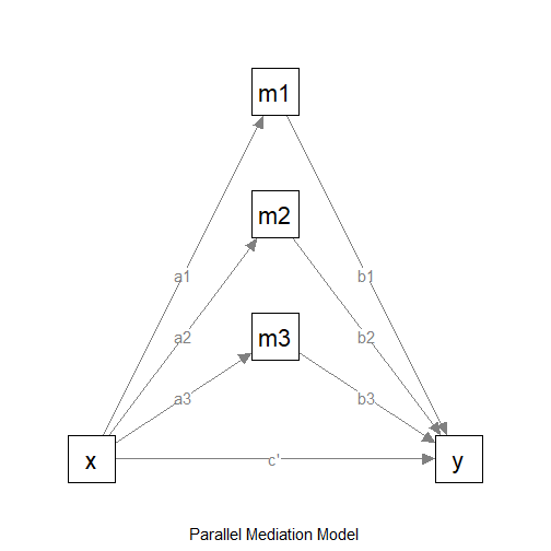
The Model
We want to do power analysis for the indirect effects from
x to y: x->m1->y,
x->m2->y, and x->m2->y. Suppose
these are the expected effects:
x->m1: smallx->m2: mediumx->m3: mediumm1->y: largem2->y: mediumm3->y: largex->y: nil (no effect)
In power4mome, the convention for Pearson’s r
is used just for convenience. If necessary, users can specify the effect
(on the standardized metric) directly.
Convention for the Effect Sizes
To make it easy to specify the standardized population values of
parameters, power4mome
adopted the convention for Pearson’s r, just for
convenience.
"nil": Nil (.00)."s": Small (.10)."m": Medium (.30),"l": Large (.50).
There are also two intermediate levels:
"sm": Small-to-medium (.20)."ml": Medium-to-large (.40).
If the effect is negative, just add a minus sign. For example, use
"-m" to denote a negative medium effect.
For a path from one variable to another variable, the standardized coefficient is equal to the correlation if there are not other predictor, or if this predictor is uncorrelated with all other predictors. Therefore, though may not be perfect, we believe the convention of Pearson’s r is a reasonable one.
If necessary, users can specify the effect (on the standardized metric) directly.
Covariates in the Model to be Fitted
In applied research, the model to be fitted usually have other
control variables, such as educational level. It may not be practical to
specify all the probable effects of these control variables (though it
is possible in power4mome).
Therefore, as a conservative assessment of power, users can first
decide the population effects, and then adjust them slightly downward
(e.g., from medium, "m", to small-to-medium,
"sm") to take into account potential decrease in effects
due to control variables to be included.
Model with Hypothesized Path Coefficients
This is the model with the effect sizes:
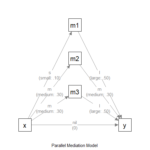
The Model (with Effect Sizes)
Omnibus Power for All Indirect Paths
There are more than one indirect path, so there are more than one
tests. The function in power4mome supports finding the
power for detecting all the indirect paths, that is, the
probability that all the tests of indirect effects are
significant. We call this power the omnibus power for the
indirect paths.
Test to be Used
In practice, nonparametric bootstrapping is usually used to test
indirect effects. However, estimating its power using simulation is
slow. A good-enough proxy is to estimate the power when testing this
effect by Monte Carlo confidence interval. This is the default method in
power4mome
for tests of indirect effects.
Find the Power
To estimate the power for a sample size, this is the code:
out_power <- q_power_mediation_parallel(
  as = c("s", "m", "m"),
  bs = c("l", "m", "l"),
  cp = "nil",
  nrep = 600,
  n = 400,
  R = 1000,
  seed = 1234
)
These are the arguments:
as: The hypothesized standardized effects from the predictorxto each mediator. This should be a character vector with elements equal to the number of mediators for the path coefficientsx->m1,x->m2, up tox->mk,kbeing the number of mediators. Can be one of the labels supported by the convention, or a numeric value.bs: The hypothesized standardized effects from each mediator to the outcome variabley. This should be a character vector with elements equal to the number of mediators for the path coefficientsm1->y,m2->y, up tomk->y,kbeing the number of mediators. Can be one of the labels supported by the convention, or a numeric value.cp: The hypothesized standardized direct effect from the predictorxto the outcome variabley. Can be one of the labels supported by the convention, or a numeric value.nrep: The number of replications when estimating the power for a sample size. Default is 400. For a crude estimate, 600 or 800 is sufficient. For the candidate sample size to be used, set it to 2000 or even 5000 for a more precise estimate of the power.R: The number of random samples used in forming Monte Carlo or nonparametric bootstrapping confidence intervals. Although they should be large when testing an effect in one single sample, they can be smaller because the goal is to estimate power across replications, not to achieve high accuracy in each sample. Default is 1000. Can be omitted if the default is acceptable.seed: The seed for the random number generator. Note that, if parallel processing is used (this is the default), then the results are reproducible only if the configuration is exactly identical. Moreover, changes in the algorithm will also make results not reproducible even with the same seed. Nevertheless, it is still advised to set this seed to an integer, to make the results reproducible at least on the same machine and version ofpower4mome. For a moderate to smallnrep, the results may be sensitive to theseed. It is advised to do a final check of the sample size to be used using annrepof 2000 or 5000.
This is the output:
out_power
#>
#> ========== power4test Results ==========
#>
#>
#> ====================== Model Information ======================
#>
#> == Model on Factors/Variables ==
#> m1 ~ x
#> m2 ~ x
#> m3 ~ x
#> y ~ m1 + m2 + m3 + x
#> == Model on Variables/Indicators ==
#> m1 ~ x
#> m2 ~ x
#> m3 ~ x
#> y ~ m1 + m2 + m3 + x
#> ====== Population Values ======
#>
#> Regressions:
#>                    Population
#>   m1 ~
#>     x                 0.100
#>   m2 ~
#>     x                 0.300
#>   m3 ~
#>     x                 0.300
#>   y ~
#>     m1                0.500
#>     m2                0.300
#>     m3                0.500
#>     x                 0.000
#>
#> Variances:
#>                    Population
#>    .m1                0.990
#>    .m2                0.910
#>    .m3                0.910
#>    .y                 0.359
#>     x                 1.000
#>
#> (Computing indirect effects for 4 paths ...)
#>
#> == Population Conditional/Indirect Effect(s) ==
#>
#> == Indirect Effect(s) ==
#>
#>                ind
#> x -> m1 -> y 0.050
#> x -> m2 -> y 0.090
#> x -> m3 -> y 0.150
#> x -> y       0.000
#>
#>  - The 'ind' column shows the indirect effect(s).
#>
#> ======================= Data Information =======================
#>
#> Number of Replications:  600
#> Sample Sizes:  400
#>
#> Call print with 'data_long = TRUE' for further information.
#>
#> ==================== Extra Element(s) Found ====================
#>
#> - fit
#> - mc_out
#>
#> === Element(s) of the First Dataset ===
#>
#> ============ <fit> ============
#>
#> lavaan 0.6-21 ended normally after 1 iteration
#>
#>   Estimator                                         ML
#>   Optimization method                           NLMINB
#>   Number of model parameters                        11
#>
#>   Number of observations                           400
#>
#> Model Test User Model:
#>
#>   Test statistic                                 4.432
#>   Degrees of freedom                                 3
#>   P-value (Chi-square)                           0.218
#>
#> =========== <mc_out> ===========
#>
#>
#> == A 'mc_out' class object ==
#>
#> Number of Monte Carlo replications: 1000
#>
#>
#> ============== <test_indirects: x-...->y> ==============
#>
#> Mean(s) across replication:
#>           test_label  est cilo cihi pvalue   sig
#> 1 x-...->y (All sig)  NaN  NaN  NaN  0.156 0.505
#>
#> - The column 'sig' shows the rejection rates.
#> - If the null hypothesis is false, the rate is the power.
#> - Number of valid replications for rejection rate(s): 600
#> - Proportion of valid replications for rejection rate(s): 1.000
#>
#> ========== power4test Power ==========
#>
#> [test]: test_indirects: x-...->y
#> [test_label]: x-...->y (All sig)
#>    est   p.v reject r.cilo r.cihi
#> 1  NaN 1.000  0.505  0.465  0.545
#> Notes:
#> - p.v: The proportion of valid replications.
#> - est: The mean of the estimates in a test across replications.
#> - reject: The proportion of 'significant' replications, that is, the
#>   rejection rate. If the null hypothesis is true, this is the Type I
#>   error rate. If the null hypothesis is false, this is the power.
#> - r.cilo,r.cihi: The confidence interval of the rejection rate, based
#>   on Wilson's (1927) method.
#> - Refer to the tests for the meanings of other columns.
The first set of output is the default printout of the output of
power4test(). This can be used to check the model
specified. It also automatically computes the population standardized
indirect effect(s).
The second section is the output of rejection_rates(),
showing the power under the column reject.
In this example, the power is about 0.50 for sample size 400, 95% confidence interval [0.47, 0.54].
Find the Sample Size with the Target Power
It is also possible to estimate the sample size with the target level
of power. This can be done by trying different sample sizes. However, if
a high level of precision is desired and so a large number of
replications (nrep), say 2000, is needed.
An alternative way is find the probable sample size using an
algorithm. This can be done with mode = "n", to find the
n (sample size). By default, the probabilistic bisection
algorithm by Waeber et al. (2013) is used.
See Chalmers (2024) for an introduction on
using this algorithm for power analysis (note
that the original algorithm by Waeber et al., 2013, is used in
power4mome).
Finding the sample size with the target level of power can be done
using the same code above, with the argument mode = "n"
added, and a few more arguments:
out_n <- q_power_mediation_parallel(
  as = c("s", "m", "m"),
  bs = c("l", "m", "l"),
  cp = "nil",
  target_power = .80,
  x_interval = c(50, 2000),
  R = 199,
  final_nrep = 2000,
  final_R = 2000,
  seed = 1234,
  mode = "n"
)
These are the arguments for this mode:
target_power: The target level of power. Default is .80, and can be omitted if this is the desired level of power.n: This is the initialn. Its value does not matter because the search will be based on an initial interval (x_interval). It can be omitted whenmodeis"n".x_interval: The interval of sample sizes to search. Default is 50 to 2000 and so this argument can be omitted is this range is desired. For the default algorithm, it is preferable to have a wide initial range. (If the model may be difficult to fit for a small sample size, increase the lower limit to a value large enough for the model.)nrep: This argument is not necessary and should be omitted.R: Set this number of a value supported by the method proposed by Boos & Zhang (2000) for the desired level of confidence (95% by default). The first few values are 39, 79, 119, 159, and 199. 199 is recommended to balance speed and accuracy.final_nrep: The desired number of replication. The search will use a much smaller value fornrep. However, the probable solution will be checked using this number of replications. a sample size will be returned as a solution only if it is close enough totarget_powerbased on this number of replications.final_R: Although the search can use a much small value forRdue to the method by Boos & Zhang (2000), users may want a larger number ofRfor the solution. To do this, setfinal_Rto theRto be used in the checking a candidate sample size.mode: Settingmodeto"n"enables this mode.
Note that this process can take a some time, sometimes more than 10 minutes. Nevertheless, power analysis is usually conducted in the planning stage of a study, and so the slow processing time is acceptable in this stage.
This is the printout, showing only the section from the output of
n_from_power():
#> ========== n_from_power Results ==========
#>
#>
#>                                      Setting
#> Predictor(x):                    Sample Size
#> Parameter:                               N/A
#> goal:                           close_enough
#> what:                                  point
#> algorithm:           probabilistic_bisection
#> Level of confidence:                  95.00%
#> Target Power:                          0.800
#>
#> - Final Value of Sample Size (n): 809
#>
#> - Final Estimated Power (CI): 0.810 [0.792, 0.827]
#>
#> Call `summary()` for detailed results.
In this example, the estimated sample size with power equal to (close to) the target level (0.80) is 809.
Based on 2000 replications, determined by final_rep, the
estimated power for 809 is 0.810, 95% confidence interval [0.792,
0.827].
How is Being “Close Enough” Defined
Being “Close enough” is defined by the tolerance value, which is
determined internally based on the number of replications
(final_nrep). For a smaller value of
final_rep, the tolerance will be larger, and so a sample
with estimated power farther away from the target power would be
considered as “close enough.” For a final_nrep of 2000, the
default tolerance is 0.018, which should be practically precise
enough.
Find the Region of Sample Sizes
If it is not necessary to have a high precision to find the sample size with the target power, we can find an approximate region of sample sizes with levels of power not significantly different from the target power. This region is useful for determining a range of sample sizes likely to have sufficient power, but are not greater than necessary when resources are limited.
Note that, unlike mode "n", this process use bisection
by default, and so the number of replications used in each trial
(iteration) need to be close to the desired final level of replication.
Therefore, this process can sometimes be very fast, but sometimes can be
slow. Again, power analysis is usually conducted in the planning stage
of a study, and so the slow processing time may be acceptable in this
stage.
Finding the region can be done using the same code for estimating
power (mode "power"), with only the argument
mode = "region" added:
out_region <- q_power_mediation_parallel(
  as = c("s", "m", "m"),
  bs = c("l", "m", "l"),
  cp = "nil",
  target_power = .80,
  nrep = 600,
  n = 400,
  R = 1000,
  seed = 1234,
  mode = "region"
)
These are the arguments for this mode:
target_power: The target level of power. Default is .80, and can be omitted if this is the desired level of powern: This is the initialn. For bisection, this will affect the search because the initial interval will be estimated based on this value Nevertheless, even if this sample size’s power is very different from the target power, the search should still be able to find the target region, though may be slower. If omitted, it will be determined internally.nrep: This number of replications will be used for all iterations. Therefore, this should not be a large value, unlike mode"n".R: For bisection, this value will be used for all iterations.mode: Settingmodeto"region"enables this mode.
This is the printout, showing only the section from the output of
n_region_from_power():
#> ========== n_region_from_power Results ==========
#>
#> Call:
#> n_region_from_power(object = `<hidden>`, target_power = 0.8,
#>     progress = TRUE, simulation_progress = NULL, max_trials = NULL,
#>     seed = 1234, algorithm = NULL)
#>
#>                      Setting
#> Predictor(x)         Sample Size
#> Goal:                Power significantly below or above the target
#> algorithm:           bisection
#> Level of confidence: 95.00%
#> Target Power:        0.800
#>
#> Solution:
#>
#> Approximate region of sample sizes with power:
#> - not significantly different from 0.800: 727 to 839
#> - significantly lower than 0.800: 727
#> - significantly higher than 0.800: 839
#>
#> Confidence intervals of the estimated power:
#> - for the lower bound (727): [0.716, 0.785]
#> - for the upper bound (839): [0.807, 0.866]
#>
#> Call `summary()` for detailed results.
In this example, the range of the sample size is 727 to 839.
The large the nrep, the higher the precision and so the
narrower this region. However, it will also take longer to run.
The results can also be visualized using the plot()
function:
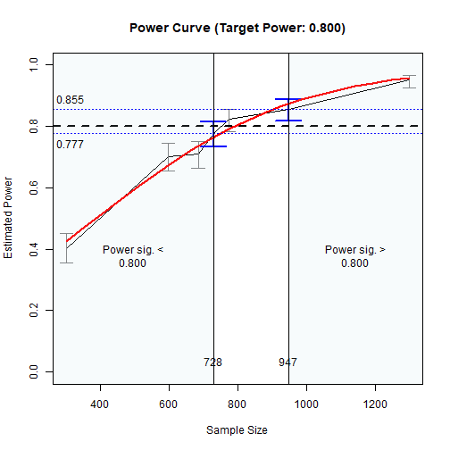
The Plot of Sample Sizes Searched
The region between the shaded areas is the approximate region of sample sizes found.
Final Remarks
Other Models
Quick how-to articles on other common mediation models, including those with latent variables, can be found from the list of articles
The package power4mome
supports an arbitrary model specified by lavaan syntax,
including those with moderators. Interested users can refer to the
articles above.
Technical Details
For options of power4test(),
n_from_power(), and n_region_from_power(),
please refer to their help pages, as well as the Get-Started
article and this article
for n_from_power(), which is also the function to find one
of the regions, called twice by n_region_from_power().