Sample Size Determination with Nonnormal Variables: Latent Variable Models
2026-03-16
Source:vignettes/articles/n_from_power_mediation_mlr_lav_simple.Rmd
n_from_power_mediation_mlr_lav_simple.RmdIntroduction
This article illustrates how to do power analysis and sample size
determination in some typical latent variable models, with the variables
hypothesized to be nonnormally distributed and the model to be estimated
using robust methods such as MLR in lavaan. The package power4mome will be
used for illustration.
Prerequisite
Basic knowledge about fitting models by lavaan and
power4mome is required.
This file is not intended to be an introduction on how to use
functions in power4mome. For details on how to use
power4test(), refer to the Get-Started
article. Please also refer to the help page of
n_region_from_power(), and the article
on n_from_power(), which is called twice by
n_region_from_power() to find the regions described
below.
Scope
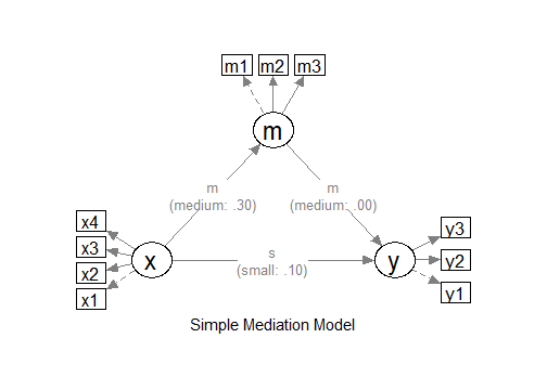
A simple mediation model of latent variables will be used as an example. Users new to the package are recommended to read the article on the steps for a model with variables having a multivariate normal distribution (the default).
Set Up the Model and Test
Load the packages first:
Estimate the power for a sample size.
The code for the model:
model <-
"
m ~ x
y ~ m + x
"

model_es <-
"
m ~ x: m
y ~ m: m
y ~ x: s
"
The Model
Refer to this article on how to
set number_of_indicators and reliability when
calling power4test().
Specify the Distributions
Suppose that we expect the error terms of the indicators are not normally distributed. For example, they represent attributes that are positively skewed, with people likely to be below the mean while some cases are far away from the mean. Without real data, it is difficult to know the actual distribution. Nevertheless, we can select a distribution that reasonably approximate the expected distribution of the error terms.
Built-In Functions For Random Numbers
The package power4mome comes with
some ready-to-use function for generating random error. A full list of
them can be found here. To be used
in power4test(), these functions need to have the
distribution standardized such that the population mean and standard
deviation are 0 and 1, respectively. All the build-in functions already
have the distributions standardized.
For example, the function rexp_rs() can be used to
approximate a heavily positively skewed distribution. The function used
is stats::rexp() from base R, but, by default, the
distribution is transformed such that the population mean and standard
deviation are 0 and 1, respectively.
An Example
Suppose we would like to estimate the power to test the indirect
effect using Monte Carlo confidence interval. We expect that the
indicators are nonnormally distributed. For the sake of illustration,
the following distributions hypothesized for the indicators of
x, m, and y.
The Indicators of x
For the indicators of x, the distribution is severely
positively skewed, generated from a lognormal distribution using
rlnorm_rs(). This is an illustration of the
distribution:
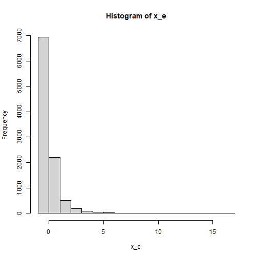
plot of chunk x_dist
The Indicators of m
The distribution of the error terms of m is assumed to
be positively skewed, but not as severe as that of x. We
use rexp_rs() to simulate this distribution:
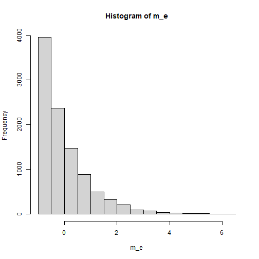
plot of chunk m_dist
The Indicators of y
Last, let’s assume that the distribution of the error terms the
indicators of y is bounded and is bimodal. We we
rbeta_rs() to simulate this distribution, setting the
parameters shape1 and shape2 to create the
bimodal distribution:
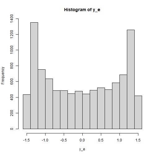
plot of chunk y_dist
In real data, we may not have a situation as complicated as this one. For example, all error terms are assumed to be normally distributed, except for the indicators of one or two latent factor. These distributions are used just to illustrate how to use the arguments.
Set the Distributions of Error Terms by e_fun
This section illustrates how to set up the call to
power4test(), with error terms generated using the
distributions described above. We would like to check the model first.
Therefore, the test of indirect effect is not added for now.
out <- power4test(
  nrep = 600,
  model = model,
  pop_es = model_es,
  n = 100,
  number_of_indicators = c(x = 4,
                           m = 3,
                           y = 3),
  reliability = c(x = .80,
                  m = .70,
                  y = .80),
  e_fun = list(x = list(rlnorm_rs),
               m = list(rexp_rs),
               y = list(rbeta_rs, shape1 = .5, shape2 = .5)),
  iseed = 1234,
  parallel = TRUE)
How to Use e_fun
The argument e_fun is used to specify the function used
to generate the error terms of indicators.
The value must be a named list, with the name being one of the latent
variables (x, m, and y in this
example).
Each element must itself a list, with the first argument is the function to be used.
- For example,
m = list(rexp_rs)indicates that the functionrexp_rswill be used to generate the error terms ofm.
If there are additional arguments to be passed to this function, include them as named arguments in the list.
- For example,
y = list(rbeta_rs, shape1 = .5, shape2 = .5)indicates thatrbeta_rswill be used to generate the error terms, and the argumentsshape1andshape2will both be set .5.
If a latent factor is not included in the list for
e_fun, the default distribution used a normal
distribution.
Functions That e_fun Can Use
In principle, any function can be used to generate the numbers for the error terms, as long as it meets these requirements:
It has an argument named
n, the number of random numbers to be generated.It returns a numeric vector.
Though no error will be returned, to ensure that the population
standardized coefficients are of the specified values, the function for
e_fun should generate numbers from a population with mean
and standard deviation equal to 0 and 1, respectively.
Check The Generated Data
To print the details of the generated data, including the descriptive
statistics, use print with
data_long = TRUE:
print(out,
      data_long = TRUE)
This is part of the output:
#> ==== Descriptive Statistics ====
#>
#>    vars     n  mean   sd  skew kurtosis se
#> x1    1 60000 -0.01 0.99  1.79    14.19  0
#> x2    2 60000  0.00 1.01  2.07    17.93  0
#> x3    3 60000  0.00 0.99  1.86    15.48  0
#> x4    4 60000  0.00 1.03  3.10    54.15  0
#> m1    5 60000  0.00 1.00  0.82     1.80  0
#> m2    6 60000  0.00 1.00  0.84     1.88  0
#> m3    7 60000  0.00 0.99  0.79     1.59  0
#> y1    8 60000  0.00 1.00 -0.01    -0.29  0
#> y2    9 60000 -0.01 1.00 -0.01    -0.27  0
#> y3   10 60000  0.00 1.00  0.01    -0.27  0
The descriptive statistics shows that the distributions of the
indicators are not normal. As expected, those of x and
m are positively skewed, while those of y are
nearly symmetric but light tailed.
Note that, the distribution of an indicator depends on both the
latent factors and and the error terms, as well as the factor loadings.
For example, the distributions of the error terms of m are
less skewed than that of an exponential distribution because the latent
factor, m, is normally distributed.
Fit the Model by MLR (Robust Maximum Likelihood)
Because of the nonnormal distribution, we would like to estimate the
power when a robust estimation method is used. One common method used in
lavaan is MLR. Although this method and the default,
maximum likelihood (ML), yield the same point estimates, their standard
errors are different. Therefore, the results from Monte Carlo confidence
intervals are also different.
The argument fit_model_args can be use to pass
arguments, as a named list, to the fit function, which is
lavaan::sem() by default.
To use MLR in lavaan::sem(), we use
estimator = "MLR". Therefore, we add the argument
fit_model_args = list(estimator = "MLR") in the call to
power4test():
out <- power4test(
  nrep = 600,
  model = model,
  pop_es = model_es,
  n = 100,
  number_of_indicators = c(x = 4,
                           m = 3,
                           y = 3),
  reliability = c(x = .80,
                  m = .70,
                  y = .80),
  e_fun = list(x = list(rlnorm_rs),
               m = list(rexp_rs),
               y = list(rbeta_rs, shape1 = .5, shape2 = .5)),
  fit_model_args = list(estimator = "MLR"),
  iseed = 1234,
  parallel = TRUE)
We can verify that MLR is used by printing the results:
print(out)This is part of the output:
#> ============ <fit> ============
#>
#> lavaan 0.6-21 ended normally after 30 iterations
#>
#>   Estimator                                         ML
#>   Optimization method                           NLMINB
#>   Number of model parameters                        23
#>
#>   Number of observations                           100
#>
#> Model Test User Model:
#>                                               Standard      Scaled
#>   Test Statistic                                22.444      23.597
#>   Degrees of freedom                                32          32
#>   P-value (Chi-square)                           0.895       0.859
#>   Scaling correction factor                                  0.951
#>     Yuan-Bentler correction (Mplus variant)
As shown in the printout, MLR was used and so there is a column
Scaled in the printout of lavaan.
Add the Test and Estimate Power
We now can add the test and estimate power. See this article
for details on the test function test_indirect_effect() and
how to set the argument test_fun and
test_args. R_for_bz(200) is used to set
R to the largest value less than 200 that is supported by
the method proposed by Boos & Zhang
(2000). 1
out <- power4test(
  nrep = 600,
  model = model,
  pop_es = model_es,
  n = 100,
  number_of_indicators = c(x = 4,
                           m = 3,
                           y = 3),
  reliability = c(x = .80,
                  m = .70,
                  y = .80),
  e_fun = list(x = list(rlnorm_rs),
               m = list(rexp_rs),
               y = list(rbeta_rs, shape1 = .5, shape2 = .5)),
  fit_model_args = list(estimator = "MLR"),
  R = R_for_bz(200),
  ci_type = "mc",
  test_fun = test_indirect_effect,
  test_args = list(x = "x",
                   m = "m",
                   y = "y",
                   mc_ci = TRUE),
  iseed = 1234,
  parallel = TRUE)
The rejection rate (power) for this example can be found by
rejection_rates():
rejection_rates(out)
#> [test]: test_indirect: x->m->y
#> [test_label]: Test
#>     est   p.v reject r.cilo r.cihi
#> 1 0.098 0.993  0.244  0.212  0.281
#> Notes:
#> - p.v: The proportion of valid replications.
#> - est: The mean of the estimates in a test across replications.
#> - reject: The proportion of 'significant' replications, that is, the
#>   rejection rate. If the null hypothesis is true, this is the Type I
#>   error rate. If the null hypothesis is false, this is the power.
#> - Some or all values in 'reject' are estimated using the extrapolation
#>   method by Boos and Zhang (2000).
#> - r.cilo,r.cihi: The confidence interval of the rejection rate, based
#>   on Wilson's (1927) method.
#> - Wilson's (1927) method is used to approximate the confidence
#>   intervals of the rejection rates estimated by the method of Boos and
#>   Zhang (2000).
#> - Refer to the tests for the meanings of other columns.
Using e_fun in Other Functions
Other functions that make use of power4test() can also
use the arguments e_fun and
fit_model_args.
For example, the output above, with nonnormal indicators, can be used
directly by n_from_power() to find a sample size given a
target power:
n_power <- n_from_power(
              out,
              target_power = .80,
              x_interval = c(100, 2000),
              final_nrep = 2000,
              seed = 1357
            )
The output with nonnormal indicators can also be used directly by
n_power_region() to find a region of sample sizes given a
target power:
n_power_region <- n_region_from_power(
                      out,
                      seed = 1357
                    )
The quick functions, described in these articles, also
support the e_fun and fit_model_args
arguments. They are set in the same way as in
power4test()
This is an example for estimating the power for a specific sample size:
q_power <- q_power_mediation_simple(
  a = "m",
  b = "m",
  cp = "s",
  number_of_indicators = c(x = 4,
                           m = 3,
                           y = 3),
  reliability = c(x = .80,
                  m = .70,
                  y = .80),
  e_fun = list(x = list(rlnorm_rs),
               m = list(rexp_rs),
               y = list(rbeta_rs, shape1 = .5, shape2 = .5)),
  fit_model_args = list(estimator = "MLR"),
  target_power = .80,
  nrep = 600,
  n = 100,
  R = R_for_bz(200),
  seed = 1234
)
This is an example of finding a sample size given a target power
(mode "n"):
q_power_n <- q_power_mediation_simple(
  a = "m",
  b = "m",
  cp = "s",
  number_of_indicators = c(x = 4,
                           m = 3,
                           y = 3),
  reliability = c(x = .80,
                  m = .70,
                  y = .80),
  e_fun = list(x = list(rlnorm_rs),
               m = list(rexp_rs),
               y = list(rbeta_rs, shape1 = .5, shape2 = .5)),
  fit_model_args = list(estimator = "MLR"),
  target_power = .80,
  R = R_for_bz(200),
  x_interval = c(100, 2000),
  final_nrep = 2000,
  seed = 1234,
  mode = "n"
)