Power Analysis for Latent Variable Mediation
2026-03-10
Source:vignettes/power4test_latent_mediation.Rmd
power4test_latent_mediation.RmdIntroduction
This article is a brief illustration of how to use
power4test() from the package power4mome to do power
analysis for the mediation effect among latent factors in a model to be
fitted by structural equation model modeling using
lavaan.
Prerequisite
Basic knowledge about fitting models by lavaan is
required. Readers are also expected to have basic knowledge of mediation
and structural equation modeling.
Scope
To make this vignette self-contained, some sections from
vignette("power4mome") are repeated here.
To do power analysis for a mediation effect in a path model with no
latent factors, please refer to vignette("power4mome").
Workflow
Two functions are sufficient for estimating power given a model, population values, sample size, and the test to be used. This is the workflow:
Specify the model syntax for the population model, in
lavaanstyle, and set the population values of the model parameters.Call
power4test()to examine the setup and the datasets generated. Repeat this and previous steps until the model is specified correctly.Call
power4test()again, with the test to do specified.Call
rejection_rates()to compute the power.
Mediation
Let’s consider a simple mediation model with three factors. We would like to estimate the power of testing the mediation effect by Monte Carlo confidence interval.
Specify the Population Model
For a model with latent factor, we only need to specify the model syntax for the factors. No need to include the measurement part and the indicators.
This is the model syntax:
mod <-
"
fm ~ fx
fy ~ fm + fx
"
The latent variables are fx, fm, and
fy. There is an indirect path from fx to
fy, through fm.
Note that, even if we are going to test a mediation effect, we do not
need to add any labels to this model. This will be taken care of by the
test functions, through the use of the package manymome
(Cheung & Cheung, 2024).
Specify The Population Values
There are two approaches to do this:
Using named vectors or lists.
Using a multiline string similar to
lavaanmodel syntax.
The second approach is demonstrated below.
Suppose we want to estimate the power when:
The path from
fxtofmare “large” in strength.The path from
fmtofyare “large” in strength.The path from
fxtofmare “small” in strength.
By default, power4mome use this convention for
regression path and correlation:1
Small: .10 (or -.10)
Medium: .30 (or -.30)
Large: .50 (or -.50)
All these values are for the standardized solution (the correlations and so-called “betas”).
The following string denotes the desired values:
mod_es <-
"
fm ~ fx: l
fy ~ fm: l
fy ~ fx: s
"
Each line starts with a tag, which is the parameter
presented in lavaan syntax. The tag ends with a colon,
:.
After the colon is population value, which can be:
-
A string denoting the value. By default:
s: Small. (-sfor small and negative.)m: Medium. (-mfor medium and negative.)l: Large. (-lfor large and negative.)nil: Zero.
All other regression coefficients and covariances, if not specified in this string, are set to zero.
Specify the Measurement Part
Power analysis is usually conducted before data collection. We rarely know in advance the factor loadings of all items. For the purpose of power analysis, which is not intended to be conducted with the knowledge of all factor loadings, we believe that, instead of specifying all the loadings, it is sufficient to specify two values for each factor:
The number of indicators.
The population reliability.
This is the approach used in power4mome.
For each factor, the population standardized factor loadings for each indicator will be derived automatically from the hypothesized (or expected) population reliability and the number of indicators, assuming that all indicators have equal loadings.
Although the equal-loading assumption is unrealistic, in a priori power analysis, it is difficult, if not impossible, to specify the pattern of factor loadings. This level of details is also not necessary because the power estimated is merely used to guide the planning of data collection, instead of estimating the “true” power after data is collected.
Two arguments will be used to set the number of indicators and the reliability.
number_of_indicators: This should be a named vector of the number of indicators for each factor. The names are the names of the factors as appeared in the model syntax, and the values are the number of indicators.reliability: This should be a named vector of the reliability for each factor. The names are the names of the factors as appeared in the model syntax, and the values are population reliability.
For example, suppose we will use the following vectors:
k <- c(fm = 3,
       fx = 4,
       fy = 5)
mod_rel <- c(fy = .70,
             fm = .60,
             fx = .50)
The numbers of indicators for fx, fm, and
fy are 4, 3, and 5, respectively.
The population reliability coefficients for fx,
fm, and fy are .50, .60, and .70,
respectively. In real research, reliability as low as .50 can be
problematic. We chose these values merely for illustration
The orders are intentionally arbitrary, to demonstrate the order does not matter. The names will be used to interpret the numbers correctly.
Call power4test() to Check the Model
We are all set and can call power4test() to check the
model:
out <- power4test(nrep = 2,
                  model = mod,
                  pop_es = mod_es,
                  number_of_indicators = k,
                  reliability = mod_rel,
                  n = 50000,
                  iseed = 1234)
These are the arguments used:
nrep: The number of replications. In this stage, a small number can be used. It is more important to have a large sample size than to have many replications.model: The model syntax.pop_es: The string setting the population values.number_of_indicators: A named vector of the number of indicators for each factor, described in the previous section.reliability: A named vector of the population reliability for each factor, described in the previous section.n: The sample size in each replications. In this stage, just for checking the model and the data generation, this number can be set to a large one unless the model is slow to fit when the sample size is large.iseed: If supplied, it is used to set the seed for the random number generator. It is advised to always set this to an arbitrary integer, to make the results reproducible.2
The population values can be shown by printing this object:
out
#>
#> ====================== Model Information ======================
#>
#> == Model on Factors/Variables ==
#>
#> fm ~ fx
#> fy ~ fm + fx
#>
#> == Model on Variables/Indicators ==
#>
#> fm ~ fx
#> fy ~ fm + fx
#>
#> fm =~ fm1 + fm2 + fm3
#> fy =~ fy1 + fy2 + fy3 + fy4 + fy5
#> fx =~ fx1 + fx2 + fx3 + fx4
#> ====== Population Values ======
#>
#> Regressions:
#>                    Population
#>   fm ~
#>     fx                0.500
#>   fy ~
#>     fm                0.500
#>     fx                0.100
#>
#> Variances:
#>                    Population
#>    .fm                0.750
#>    .fy                0.690
#>     fx                1.000
#>
#> (Computing indirect effects for 2 paths ...)
#>
#> == Population Conditional/Indirect Effect(s) ==
#>
#> == Indirect Effect(s) ==
#>
#>                  ind
#> fx -> fm -> fy 0.250
#> fx -> fy       0.100
#>
#>  - The 'ind' column shows the indirect effect(s).
#>
#> ==== Population Reliability ====
#>
#>   fy  fm  fx
#>  0.7 0.6 0.5
#>
#> == Population Standardized Loadings ==
#>
#>    Standardized Loadings
#> fm 0.577,0.577,0.577
#> fx 0.447,0.447,0.447,0.447
#> fy 0.564,0.564,0.564,0.564,0.564
#>
#> ======================= Data Information =======================
#>
#> Number of Replications:  2
#> Sample Sizes:  50000
#>
#> Call print with 'data_long = TRUE' for further information.
#>
#> ==================== Extra Element(s) Found ====================
#>
#> - fit
#>
#> === Element(s) of the First Dataset ===
#>
#> ============ <fit> ============
#>
#> lavaan 0.6-21 ended normally after 44 iterations
#>
#>   Estimator                                         ML
#>   Optimization method                           NLMINB
#>   Number of model parameters                        27
#>
#>   Number of observations                         50000
#>
#> Model Test User Model:
#>
#>   Test statistic                                38.042
#>   Degrees of freedom                                51
#>   P-value (Chi-square)                           0.910
By the default, the population model will be fitted to each dataset,
hence the section <fit>. The fit is not “perfect”
because the model is not a saturated model. However, the
p-value is high and not significant (because, with the
population model fitted, the chance of significant is close to .05).
Although we specify only the structure for the latent factors, we can
see the automatically generated measurement part syntax in the section
Model on Variables/Indicators:
#> fm =~ fm1 + fm2 + fm3
#> fy =~ fy1 + fy2 + fy3 + fy4 + fy5
#> fx =~ fx1 + fx2 + fx3 + fx4
It confirmed that we specified the measurement part correctly.
We then check the section Population Values to see
whether the values are what we expected.
- In this example, the population values for the regression paths are what we specified.
If they are different from what we expect, check the string for
pop_es to see whether we set the population values
correctly.
- The section
Variances:shows the variances or error variances of the latent factors. Becausefmandfyare endogenous factors, the values presented, next to.fmand.fy, are error variances, and that’s why they are not 1, unlikefx.
The section Population Reliability shows the population
reliability coefficients:
#> ==== Population Reliability ====
#>
#>   fy  fm  fx
#>  0.7 0.6 0.5
They are the values we set to reliability.
The section Population Standardized Loadings shows the
standardized factor loadings for each factor. Only one value for each
factor because the loadings are assumed to be the same for all
items:
#> == Population Standardized Loadings ==
#>
#>    Standardized Loadings
#> fm 0.577,0.577,0.577
#> fx 0.447,0.447,0.447,0.447
#> fy 0.564,0.564,0.564,0.564,0.564
If necessary, we can check the data generation by adding
data_long = TRUE when printing the output:
print(out,
      data_long = TRUE)
Two new sections will be printed. This is the first one:
#> ==== Descriptive Statistics ====
#>
#>     vars     n mean   sd  skew kurtosis se
#> fm1    1 1e+05 0.00 1.00  0.01     0.00  0
#> fm2    2 1e+05 0.01 1.00  0.01    -0.01  0
#> fm3    3 1e+05 0.00 1.01  0.00    -0.02  0
#> fx1    4 1e+05 0.00 1.00  0.00     0.00  0
#> fx2    5 1e+05 0.00 1.00 -0.01     0.00  0
#> fx3    6 1e+05 0.00 1.00 -0.01    -0.02  0
#> fx4    7 1e+05 0.00 1.00  0.00     0.00  0
#> fy1    8 1e+05 0.00 1.00  0.01     0.01  0
#> fy2    9 1e+05 0.00 1.00  0.01     0.00  0
#> fy3   10 1e+05 0.00 1.00  0.00     0.01  0
#> fy4   11 1e+05 0.01 1.00  0.01     0.00  0
#> fy5   12 1e+05 0.00 1.00  0.02    -0.01  0
The section Descriptive Statistics, generated by
psych::describe(), shows basic descriptive statistics for
indicators. As expected, they have means close to zero and standard
deviations close to one, because the datasets were generated using the
standardized model.
This is the second one:
#> fy5   12 1e+05 0.00 1.00  0.02    -0.01  0
#>
#> ===== Parameter Estimates Based on All 2 Samples Combined =====
#>
#> Total Sample Size: 100000
#>
#> ==== Standardized Estimates ====
#>
#> Variances and error variances omitted.
#>
#> Latent Variables:
#>                     est.std
#>   fm =~
#>     fm1               0.578
#>     fm2               0.579
#>     fm3               0.578
#>   fy =~
#>     fy1               0.559
#>     fy2               0.560
#>     fy3               0.563
#>     fy4               0.565
#>     fy5               0.569
#>   fx =~
#>     fx1               0.445
#>     fx2               0.443
#>     fx3               0.445
#>     fx4               0.445
#>
#> Regressions:
#>                     est.std
#>   fm ~
#>     fx                0.504
#>   fy ~
#>     fm                0.505
#>     fx                0.097
The section Parameter Estimates Based on shows the
parameter estimates when the population model is fitted to
all the datasets combined. When the total sample size is large,
these estimates should be close to the population values.
The results show that we have specified the population model correctly. We can proceed to specify the test and estimate the power.
Call power4test() to Do the Target Test
We can now do the simulation to estimate power. A large number of datasets (e.g., 400) of the target sample size are to be generated, and then the target test will be conducted in each of these datasets.
Suppose we would like to estimate the power of using Monte Carlo
confidence interval to test the indirect effect from fx to
fy through fm, when sample size is 150. This
is the call:
out <- power4test(nrep = 400,
                  model = mod,
                  pop_es = mod_es,
                  number_of_indicators = k,
                  reliability = mod_rel,
                  n = 150,
                  R = 2000,
                  ci_type = "mc",
                  test_fun = test_indirect_effect,
                  test_args = list(x = "fx",
                                   m = "fm",
                                   y = "fy",
                                   mc_ci = TRUE),
                  iseed = 1234,
                  parallel = TRUE)
These are the new arguments used:
R: The number of replications used to generate the Monte Carlo simulated estimates, 2000 in this example. In real studies, this number should be 10000 or even 20000 for Monte Carlo confidence intervals. However, 2000 is sufficient because the goal is to estimate power by generating many intervals, rather than to have one single stable interval.ci_type: The method used to generate estimates. Support both Monte Carlo ("mc") and nonparametric bootstrapping ("boot").3 Although bootstrapping is usually used to test an indirect effect, it is very slow to doRbootstrapping innrepdatasets (the model will be fittedR * nreptimes). Therefore, it is preferable to use Monte Carlo to do the initial estimation.test_fun: The function to be used to do the test for each replication. Any function following a specific requirement can be used, andpower4momecomes with several built-in functions for some common tests. The functiontest_indirect_effect()is used to test an indirect effect in the model.test_args: A named list of arguments to be supplied totest_fun. Fortest_indirect_effect(), it is a named list specifying the predictor (x), the mediator(s) (m), and the outcome (y). A path with any number of mediators can be supported. Please refer to the help page oftest_indirect_effect().4parallel: If the test to be conducted is slow, which is the case for tests done by Monte Carlo or nonparametric bootstrapping confidence interval, it is advised to enable parallel processing by settingparalleltoTRUE.5
For nrep = 400, the 95% confidence limits for a power of
.80 are about .04 below and above .80. This should be precise enough for
determining whether a sample size has sufficient power. If a higher
precision is desired, set nrep to 1000 or 2000 for the
sample size to be used.
This is the default printout:
out
#>
#> ====================== Model Information ======================
#>
#> == Model on Factors/Variables ==
#>
#> fm ~ fx
#> fy ~ fm + fx
#>
#> == Model on Variables/Indicators ==
#>
#> fm ~ fx
#> fy ~ fm + fx
#>
#> fm =~ fm1 + fm2 + fm3
#> fy =~ fy1 + fy2 + fy3 + fy4 + fy5
#> fx =~ fx1 + fx2 + fx3 + fx4
#> ====== Population Values ======
#>
#> Regressions:
#>                    Population
#>   fm ~
#>     fx                0.500
#>   fy ~
#>     fm                0.500
#>     fx                0.100
#>
#> Variances:
#>                    Population
#>    .fm                0.750
#>    .fy                0.690
#>     fx                1.000
#>
#> (Computing indirect effects for 2 paths ...)
#>
#> == Population Conditional/Indirect Effect(s) ==
#>
#> == Indirect Effect(s) ==
#>
#>                  ind
#> fx -> fm -> fy 0.250
#> fx -> fy       0.100
#>
#>  - The 'ind' column shows the indirect effect(s).
#>
#> ==== Population Reliability ====
#>
#>   fy  fm  fx
#>  0.7 0.6 0.5
#>
#> == Population Standardized Loadings ==
#>
#>    Standardized Loadings
#> fm 0.577,0.577,0.577
#> fx 0.447,0.447,0.447,0.447
#> fy 0.564,0.564,0.564,0.564,0.564
#>
#> ======================= Data Information =======================
#>
#> Number of Replications:  400
#> Sample Sizes:  150
#>
#> Call print with 'data_long = TRUE' for further information.
#>
#> ==================== Extra Element(s) Found ====================
#>
#> - fit
#> - mc_out
#>
#> === Element(s) of the First Dataset ===
#>
#> ============ <fit> ============
#>
#> lavaan 0.6-21 ended normally after 38 iterations
#>
#>   Estimator                                         ML
#>   Optimization method                           NLMINB
#>   Number of model parameters                        27
#>
#>   Number of observations                           150
#>
#> Model Test User Model:
#>
#>   Test statistic                                69.181
#>   Degrees of freedom                                51
#>   P-value (Chi-square)                           0.046
#>
#> =========== <mc_out> ===========
#>
#>
#> == A 'mc_out' class object ==
#>
#> Number of Monte Carlo replications: 2000
#>
#>
#> ============= <test_indirect: fx->fm->fy> =============
#>
#> Mean(s) across replication:
#>    est   cilo  cihi   sig pvalue
#>  0.336 -0.056 0.832 0.492  0.100
#>
#> - The value 'sig' is the rejection rate.
#> - If the null hypothesis is false, this is the power.
#> - Number of valid replications for rejection rate: 400
#> - Proportion of valid replications for rejection rate: 1.000
Compute the Power
The power estimate is simply the proportion of significant results,
the rejection rate, because the null hypothesis is
false. The rejection rate can be retrieved by
rejection_rates().
out_power <- rejection_rates(out)
out_power
#> [test]: test_indirect: fx->fm->fy
#> [test_label]: Test
#>     est   p.v reject r.cilo r.cihi
#> 1 0.336 1.000  0.492  0.444  0.541
#> Notes:
#> - p.v: The proportion of valid replications.
#> - est: The mean of the estimates in a test across replications.
#> - reject: The proportion of 'significant' replications, that is, the
#>   rejection rate. If the null hypothesis is true, this is the Type I
#>   error rate. If the null hypothesis is false, this is the power.
#> - r.cilo,r.cihi: The confidence interval of the rejection rate, based
#>   on Wilson's (1927) method.
#> - Refer to the tests for the meanings of other columns.
In the example above, the estimated power of the test of the indirect
effect, conducted by Monte Carlo confidence interval, is 0.492, under
the column reject.
p.v is the proportion of valid results across
replications. 1.000 means that the test conducted normally
in all replications.
By default, the 95% confidence interval of the rejection rate (power)
based on normal approximation is also printed, under the column
r.cilo and r.cihi. In this example, the 95%
confidence interval is [0.444; 0.541].
Repeat a Simulation With A Different Sample Size
The function power4test() also supports redoing
an analysis using a new value for the sample size (or population effect
sizes set to pop_es). Simply
set the output of
power4testas the first argument, andset the new value for
n.
For example, we can repeat the simulation for the test of indirect
effect, but for a smaller sample size of 200. We simply call
power4test() again, set the previous output
(out in the example above) as the first argument, and set
n to a new value (200 in this example):
out_new_n <- power4test(out,
                        n = 200)
out_new_n
This is the estimated power when the sample size is 200.
out_new_n_reject <- rejection_rates(out_new_n)
out_new_n_reject
#> [test]: test_indirect: fx->fm->fy
#> [test_label]: Test
#>     est   p.v reject r.cilo r.cihi
#> 1 0.352 1.000  0.818  0.777  0.852
#> Notes:
#> - p.v: The proportion of valid replications.
#> - est: The mean of the estimates in a test across replications.
#> - reject: The proportion of 'significant' replications, that is, the
#>   rejection rate. If the null hypothesis is true, this is the Type I
#>   error rate. If the null hypothesis is false, this is the power.
#> - r.cilo,r.cihi: The confidence interval of the rejection rate, based
#>   on Wilson's (1927) method.
#> - Refer to the tests for the meanings of other columns.
The estimated power is 0.818, 95% confidence interval [0.777; 0.852], when the sample size is 200.
This technique can be repeated to find the required sample size for a target power.
Repeat a Simulation With Different Numbers of Indicators or Reliability
We can also redo an analysis using a new value for reliability. For example, we may want to see whether we can have a higher power if we use more reliable scales.
As in the previous example, we just call power4test()
one the original output, but set reliability to a new
vector.
Assume that we want to know the power for the same scenario, but with all scales having a population reliability of .80:
out_new_rel <- power4test(out,
                          reliability = c(fx = .80,
                                          fm = .80,
                                          fy = .80))
out_new_rel
This is the estimated power with higher population reliability:
out_new_rel_reject <- rejection_rates(out_new_rel)
out_new_rel_reject
#> [test]: test_indirect: fx->fm->fy
#> [test_label]: Test
#>     est   p.v reject r.cilo r.cihi
#> 1 0.235 1.000  0.988  0.971  0.995
#> Notes:
#> - p.v: The proportion of valid replications.
#> - est: The mean of the estimates in a test across replications.
#> - reject: The proportion of 'significant' replications, that is, the
#>   rejection rate. If the null hypothesis is true, this is the Type I
#>   error rate. If the null hypothesis is false, this is the power.
#> - r.cilo,r.cihi: The confidence interval of the rejection rate, based
#>   on Wilson's (1927) method.
#> - Refer to the tests for the meanings of other columns.
The estimated power is 0.988, 95% confidence interval [0.971; 0.995], much higher than the original scenario.
Find the Sample Size With Desired Power
There are several more efficient ways to find the sample size with the desired power.
Using n_region_from_power()
This is the recommended way for sample size planning, when there is no predetermined range of sample sizes, and time is not a concern in searching for the sample size with the target level of power.
The function n_region_from_power() can be used to find
the region of sample sizes likely to have the desired power. If
the default settings are to be used, then it can be called directly on
the output of power4test():
out2_region <- n_region_from_power(out2,
                                   seed = 2345)
See the
templates for examples on using n_region_from_power()
for common models.
Using power4test_by_n()
This approach is used when the range of sample sizes has already been decided and the levels of power are needed to determine the final sample size.
First, the function power4test_by_n() can be used To
estimate the power for a sequence of sample sizes. For example, suppose
we do not know that the power is about .80 with a sample size of 200. We
can estimate the power in the mediation model above for these sample
sizes: 175, 200, 225, 250.
out_several_ns <- power4test_by_n(out,
                                  n = c(175, 200, 225, 250),
                                  by_seed = 4567)
The first argument is the output of power4test() for an
arbitrary sample size.
The argument n is a numeric vector of sample sizes to
examine. For each n, nrep datasets will be
generated. Although there is no limit on the number of sample sizes to
try, it is recommended to restrict the number of sample sizes to 5 or
less.
The argument by_seed, if set to an integer, tries to
make the results reproducible. Note that reproducibility is always
possible due to parallel processing. Use a larger nrep to
ensure stability of the results if necessary.
The call will take some time to run because it is equivalent to
calling power4test() once for each sample size.
The rejection rates for each sample size can be retrieved by
rejection_rates() too:
rejection_rates(out_several_ns)
#> [test]: test_indirect: fx->fm->fy
#> [test_label]: Test
#>     n   est   p.v reject r.cilo r.cihi
#> 1 175 0.327 1.000  0.703  0.656  0.745
#> 2 200 0.329 1.000  0.833  0.793  0.866
#> 3 225 0.340 1.000  0.897  0.864  0.924
#> 4 250 0.330 1.000  0.907  0.875  0.932
#> Notes:
#> - n: The sample size in a trial.
#> - p.v: The proportion of valid replications.
#> - est: The mean of the estimates in a test across replications.
#> - reject: The proportion of 'significant' replications, that is, the
#>   rejection rate. If the null hypothesis is true, this is the Type I
#>   error rate. If the null hypothesis is false, this is the power.
#> - r.cilo,r.cihi: The confidence interval of the rejection rate, based
#>   on Wilson's (1927) method.
#> - Refer to the tests for the meanings of other columns.
The method plot() can also be used to plot the
results:
plot(out_several_ns)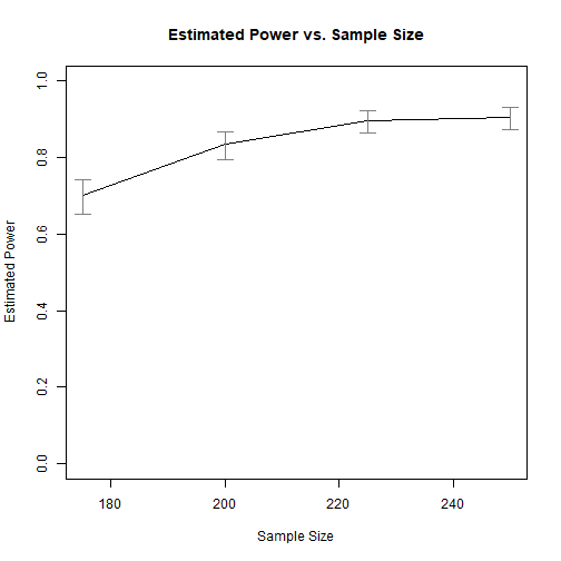
Power by Sample Size
The results show that, to have a power of about .800 to detect the mediation effect, a sample size of about 200 is needed.
Please refer to the help page of power4test_by_n() for
other examples.
Using x_from_power()
The function x_from_power() can be used to
systematically search within an interval the sample size with the target
power. This takes longer to run but, instead of manually trying
different sample size, this function do the search automatically.
This approach can be used when the goal is to find the probable
minimum or maximum sample size with the desired level of power. The
first approach, using n_region_from_power(), simply uses
this approach twice to find the region of sample sizes.
See this
article for an illustration of how to use
x_from_power().
Other Scenarios
For other scenarios, such as moderation and moderated mediation,
please refer to vignette("power4mome").