Sample Size and Effect Size Determination

It searches by simulation the sample size (given other factors, such as effect sizes) or effect size (given other factors, such as sample size) with power to detect an effect close to a target value.

Usage

x_from_power(
  object,
  x = arg_x_from_power(object, "x", arg_in = "call") %||% "n",
  pop_es_name = arg_x_from_power(object, "pop_es_name", arg_in = "call"),
  target_power = 0.8,
  what = arg_x_from_power(object, "what") %||% "point",
  goal = arg_x_from_power(object, "goal") %||% {
     switch(what, point = "ci_hit", ub
    = "close_enough", lb = "close_enough")
 },
  ci_level = 0.95,
  tolerance = NULL,
  x_interval = switch(x, n = c(50, 2000), es = NULL),
  extendInt = NULL,
  progress = TRUE,
  simulation_progress = NULL,
  max_trials = NULL,
  final_nrep = attr(object, "args")$nrep %||% (object$nrep_final %||% 400),
  final_R = attr(object, "args")$R %||% (object$args$final_R %||% 1000),
  seed = NULL,
  x_include_interval = FALSE,
  check_es_interval = TRUE,
  power_curve_args = list(power_model = NULL, start = NULL, lower_bound = NULL,
    upper_bound = NULL, nls_control = list(), nls_args = list()),
  save_sim_all = FALSE,
  algorithm = NULL,
  control = list(),
  internal_args = list(),
  rejection_rates_args = list(collapse = "all_sig", at_least_k = 1, p_adjust_method =
    "none", alpha = 0.05)
)

n_from_power(
  object,
  pop_es_name = NULL,
  target_power = 0.8,
  what = formals(x_from_power)$what,
  goal = formals(x_from_power)$goal,
  ci_level = 0.95,
  tolerance = NULL,
  x_interval = c(50, 2000),
  extendInt = NULL,
  progress = TRUE,
  simulation_progress = NULL,
  max_trials = NULL,
  final_nrep = formals(x_from_power)$final_nrep,
  final_R = formals(x_from_power)$final_R,
  seed = NULL,
  x_include_interval = FALSE,
  check_es_interval = TRUE,
  power_curve_args = list(power_model = NULL, start = NULL, lower_bound = NULL,
    upper_bound = NULL, nls_control = list(), nls_args = list()),
  save_sim_all = FALSE,
  algorithm = NULL,
  control = list(),
  internal_args = list(),
  rejection_rates_args = list(collapse = "all_sig", at_least_k = 1, p_adjust_method =
    "none", alpha = 0.05)
)

n_region_from_power(
  object,
  pop_es_name = NULL,
  target_power = 0.8,
  ci_level = 0.95,
  tolerance = NULL,
  x_interval = c(50, 2000),
  extendInt = NULL,
  progress = TRUE,
  simulation_progress = NULL,
  max_trials = NULL,
  final_nrep = formals(x_from_power)$final_nrep,
  final_R = formals(x_from_power)$final_R,
  seed = NULL,
  x_include_interval = FALSE,
  check_es_interval = TRUE,
  power_curve_args = list(power_model = NULL, start = NULL, lower_bound = NULL,
    upper_bound = NULL, nls_control = list(), nls_args = list()),
  save_sim_all = FALSE,
  algorithm = NULL,
  control = list(),
  internal_args = list(),
  rejection_rates_args = list(collapse = "all_sig", at_least_k = 1, p_adjust_method =
    "none", alpha = 0.05)
)

# S3 method for class 'x_from_power'
print(x, digits = 3, call = TRUE, ...)

# S3 method for class 'n_region_from_power'
print(x, digits = 3, ...)

arg_x_from_power(object, arg, arg_in = NULL)

pba_diagnosis(
  a_out,
  p_interval = c(0.05, 0.95),
  posterior_xlim = c(0.01, 0.99),
  which = NULL
)

Arguments

object

A power4test object, which is the output of power4test(). Can also be a power4test_by_n object, the output of power4test_by_n(), or a power4test_by_es object, the output of power4test_by_es(). For these two types of objects, the attempt with power closest to the target_power will be used as object, and all other attempts in them will be included in the estimation of subsequent attempts and the final output. Last, it can also be the output of a previous call to x_from_power(), and the stored trials will be retrieved.

x

For x_from_power(), x set the value to be searched. Can be "n", the sample size, or "es", the population value of a parameter (set by pop_es_name). For the print method of x_from_power objects, this is the output of x_from_power().

pop_es_name

The name of the parameter. Required if x is "es". See the help page of ptable_pop() on the names for the argument pop_es.

target_power

The target power, a value greater than 0 and less than one.

what

The value for which is searched: the estimate power ("point"), the upper bound of the confidence interval ("ub"), or the lower bound of the confidence interval ("lb").

goal

The goal of the search. If "ci_hit", then the goal is to find a value of x with the confidence interval of the estimated power including the target power. If "close_enough", then the goal is to find a value of x with the value in what "close enough" to the target power, defined by having an absolute difference with the target power less than tolerance.

ci_level

The level of confidence of the confidence intervals computed for the estimated power. Default is .95, denoting 95%.

tolerance

Used when the goal is "close_enough". If NULL, set automatically based on the algorithm used.

x_interval

A vector of two values, the minimum value and the maximum values of x, in the search for the values (sample sizes or population values). If NULL, default when x = "es", it will be determined internally.

extendInt

Whether x_interval can be expanded when estimating the the values to try. The value will be passed to the argument of the same name in stats::uniroot(). If x is "n", then the default value is "upX". That is, a value higher than the maximum in x_interval is allowed, if predicted by the tentative model. Otherwise, the default value is "no". See the help page of stats::uniroot() for further information.

progress

Logical. Whether the searching progress is reported.

simulation_progress

Logical. Whether the progress in each call to power4test(), power4test_by_n(), or power4test_by_es() is shown. To be passed to the progress argument of these functions. If NULL, set automatically based on the algorithm used.

max_trials

The maximum number of trials in searching the value with the target power. Rounded up if not an integer. If NULL, set automatically based on the algorithm used.

final_nrep

The number of replications in the final stage, also the maximum number of replications in each call to power4test(), power4test_by_n(), or power4test_by_es(). If object is an output of power4test() or x_from_power() and this argument is not set, final_nrep will be set to nrep or final_nrep stored in object.

final_R

The number of Monte Carlo simulation or bootstrapping samples in the final stage. The R in calling power4test(), power4test_by_n(), or power4test_by_es() will be stepped up to this value when approaching the target power. Do not need to be very large because the goal is to estimate power by replications, not for high precision in one single replication. If object is an output of power4test() or x_from_power() and this argument is not set, final_R will be set to R or final_R stored in object.

seed

If not NULL, set.seed() will be used to make the process reproducible. This is not always possible if many stages of parallel processing is involved.

x_include_interval

Logical. Whether the minimum and maximum values in x_interval are mandatory to be included in the values to be searched.

check_es_interval

If TRUE, the default, and x is "es", a conservative probable range of valid values for the selected parameter will be determined, and it will be used instead of x_interval. If the range spans both positive and negative values, only the interval of the same sign as the population value in object will be used.

power_curve_args

A named list of arguments to be passed power_curve() when estimating the relation between power and x (sample size or effect size). Please refer to power_curve() on available arguments. There is one except: power_model is mapped to the formula argument of power_curve().

save_sim_all

If FALSE, the default, the data in each power4test object for each value of x is not saved, to reduce the size of the output. If set to TRUE, the size of the output can be very large in size.

algorithm

The algorithm for finding x. Can be "power_curve", "bisection", or "probabilistic_bisection". The default algorithm depends on x.

control

A named list of additional arguments to be passed to the algorithm to be used. For advanced users.

internal_args

A named list of internal arguments. For internal testing. Do not use it.

rejection_rates_args

Argument values to be used when rejection_rates() is called, used to decide how rejection rates will be estimated. Only one single test is supported by x_from_power(). Therefore, merge_all_tests is always TRUE and cannot be changed. The argument collapse can be "all_sig", "at_least_one_sig", or "at_least_k_sig" (it cannot be "none"). Please refer to rejection_rates() for other possible arguments. These values, if set, will overwrite any stored settings in object.

digits

The number of digits after the decimal when printing the results.

call

Logical. Whether the call is printed.

...

Optional arguments. Not used for now.

arg

The name of element to retrieve.

arg_in

The name of the element from which an element is to be retrieved.

a_out

The output of x_from_power() and friends. The algorithm used must be "probabilistic_bisection".

p_interval

The range of the plot that "zooms" around the solution (or the median of in the final posterior probability distribution), expressed in terms of the area of the distribution.

posterior_xlim

The range of the first plot of search history and the plot of posterior probability distribution, expressed in terms of the area of the distribution.

which

If a_out is a list with more than one output of x_from_power(), such as the output of n_region_from_power(), which must be set to the name of one such output ("below" or "above" for the output of n_region_from_power(), or the output of q_power_mediation_*).

Value

The function x_from_power() returns an x_from_power object, which is a list with the following elements:

• power4test_trials: The output of power4test_by_n() for all sample sizes examined, or of power4test_by_es() for all population values of the selected parameter examined.

• rejection_rates: The output of rejection_rates().

• x_tried: The sample sizes or population values examined.

• power_tried: The estimated rejection rates for all the values examined.

• x_final: The sample size or population value in the solution. NA if a solution not found.

• power_final: The estimated power of the value in the solution. NA if a solution not found.

• i_final: The position of the solution in power4test_trials. NA if a solution not found.

• ci_final: The confidence interval of the estimated power in the solution. The method is determined by the option power4mome.ci_method. If NULL or "wilson", Wilson's (1927) method is used. If "norm", normal approximation is used.

• ci_level: The level of confidence of ci_final.

• nrep_final: The number of replications (nrep) when estimating the power in the solution.

• power_curve: The output of power_curve() when estimating the power curve.

• target_power: The requested target power.

• power_tolerance: The allowed difference between the solution's estimated power and the target power. Determined by the number of replications and the level of confidence of the confidence intervals.

• x_estimated: The value (sample size or population value) with the target power, estimated by power_curve. This is used, when solution not found, to determine the range of the values to search when calling the function again.

• start: The time and date when the process started.

• end: The time and date when the process ended.

• time_spent: The time spent in doing the search.

• args: A named list of the arguments of x_from_power() used in the search.

• call: The call when this function is called.

The function n_region_from_power() returns a named list of two output of n_from_power(), of the class n_region_from_power. The output with what = "ub" is named "below", and the output with what = "lb" is namd "above".

The print-method of x_from_power objects returns the object x invisibly. It is called for its side effect.

The print-method of x_from_power_region objects returns the object x invisibly. It is called for its side effect.

The function arg_x_from_power() returns the requested argument if available. If not available, it returns NULL.

The function pba_diagnosis() returns NULL invisibly. Called for its side-effect.

Details

This is how to use x_from_power():

• Specify the model by power4test(), with do_the_test = FALSE, and set the magnitude of the effect sizes to the minimum levels to detect.

• Add the test using power4test() using test_fun and test_args (see the help page of power4test() for details). Run it on the starting sample size or effect size.

• Call x_from_power() on the output of power4test() returned from the previous step. This function will iteratively repeat the analysis on either other sample sizes, or other values for a selected model parameter (the effect sizes), trying to achieve a goal (goal) for a value of interest (what).

If the goal is "ci_hit", the search will try to find a value (a sample size, or a population value of the selected model parameter) with a power level close enough to the target power, defined by having its confidence interval for the power including the target power.

If the goal is "close_enough", then the search will try to find a value of x with its level of power ("point"), the upper bound of the confidence interval for this level of power ("ub"), or the lower bound of the confidence interval fro this level of power ("lb") "close enough" to the target level of power, defined by having an absolute difference less than the tolerance.

If several values of x (sample size or the population value of a model parameter) have already been examined by power4test_by_n() or power4test_by_es(), the output of these two functions can also be used as object by x_from_power().

Usually, the default values of the arguments should be sufficient.

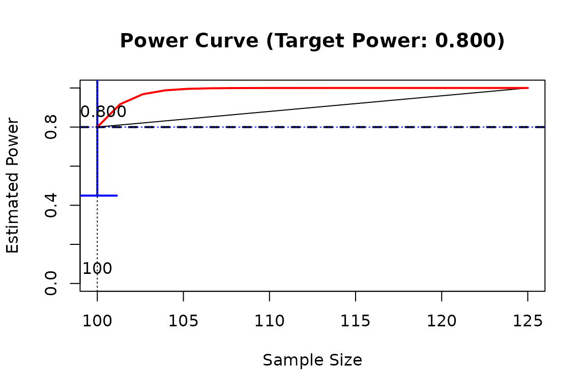
The results can be viewed using summary(), and the output has a plot method (plot.x_from_power()) to plot the relation between power and values (of x) examined.

A detailed illustration on how to use this function for sample size can be found from this page:

https://sfcheung.github.io/power4mome/articles/x_from_power_for_n.html

The function n_from_power() is just a wrapper of x_from_power(), with x set to "n".

The function n_region_from_power() is just a wrapper of x_from_power(), with x set to "n", with two passes, one with what = "ub" and one with what = "lb".

The print method only prints basic information. Call the summary method of x_from_power objects (summary.x_from_power()) and its print method for detailed results

The function arg_x_from_power() is a helper to set argument values if object is an output of x_from_power() or similar functions.

The function pba_diagnosis() generates simple diagnostic plots for the search history of probabilistic bisection algorithm. This function is for advanced users to examine the search history of the probabilistic bisection algorithm. It is for diagnostic purpose and has limited support for customizing the plots.

Algorithms

Three algorithms are currently available, the simple (though sometimes inefficient) bisection method, a method that makes use of the estimated crude power curve, and probabilistic bisection algorithm (Waeber et al., 2013; see Chalmers, 2024, for applying this algorithm to power analysis).

Unlike typical root-finding problems, the prediction of the level of power is stochastic. Moreover, the computational cost is high when Monte Carlo or bootstrap confidence intervals are used to do a test because the estimation of the power for one single value of x can sometimes take one minute or longer. Therefore, in addition to the simple bisection method, two methods, named power curve method (which belongs to the family of surrogate function approximation method reviewed in Chalmers, 2024) and probabilistic bisection method (Chalmers, 2024; Waeber et al., 2013) were also developed for this scenario.

Bisection Method

This method (called informat bisection in Chalmers, 2024), enabled by algorithm = "bisection", basically starts with an interval that probably encloses the value of x that meets the goal, and then successively narrows this interval. A point inside this interval, usually the mid-point but can also be approximated by another method (e.g., the power curve method), is used as the estimate. Though simple, there are cases in which it can be slow. Nevertheless, preliminary examination suggests that this method is good enough for scenarios in which only an approximate sample size or range of sample sizes is needed.

The internal workflow of this method implemented in x_from_power() will be presented in a forthcoming technical vignette.

Power Curve Method

This method (belongs to the surrogate function approximation family reviewed in Chalmers, 2024), enabled by algorithm = "power_curve", starts with a crude power curve based on a few points. This tentative model is then used to suggest the values to examine in the next iteration. Unlike some other implementations of this family of methods, the form, not just the parameters, of the model can change across iterations, as more and more data points are available.

This method is the default method for some scenarios, such as x = "es" with goal = "ci_hit" because the relation between the power and the population value of a parameter varies across parameters, unlike the relation between power and sample size, which is monotonic. Therefore, taking into account the working power curve may help finding the desired value of x.

Before version 0.1.1.33, this method can be used only with the goal "ci_hit". Since version 0.1.1.34, it supports all goals, like the bisection method.

The internal workflow of this method implemented in x_from_power() can be found in this technical vignette: https://sfcheung.github.io/power4mome/articles/x_from_power_workflow.html.

Probabilistic Bisection

This method, proposed by Waeber and others (2013) for stochastic root-solving, has been adapted by Chalmers (2024) for power analysis. Similar to bisection, this method starts with an interval, with a initial probability for each value (or range of values), such as sample sizes, as the sample size with the target power. A value is then selected to estimate power (the median, by default). Based on the estimated power for this value, the distribution of probabilities is updated. This process is repeated until some termination criteria are met.

Unlike bisection, each iteration can be conducted with a small number of replications (e.g., 50). The method accumulate evidence in a Bayesian approach, and so the certainty of the solution is based on the accumulation of evidence from successive iterations, not on having strong evidence from a few iterations.

In x_from_power, the version of probabilistic bisection proposed by Waeber et al. (2013) was implemented, with minor changes.

Most importantly, when some termination criteria are met, the candidate value of x (e.g., a sample size) will be checked using a larger number of replications (set by final_nrep) to ensure that the estimated power is indeed close enough to the target power (based on tolerance value, determined internally but can also be set directly). If yes, it will be returned as the solution. If no, then the search will continue, until a maximum number of candidate values has been checked.

Although the bisection method can be fast in some situations (e.g., when the interval is narrow and the solution happens to be inside the interval), the probabilistic bisection method is nearly guaranteed to converge to the solution (as long as the solution is inside the interval). Therefore, this is the default algorithm in some scenarios.

The internal workflow of this method implemented in x_from_power() will be presented in a forthcoming technical vignette.

References

Chalmers, R. P. (2024). Solving variables with Monte Carlo simulation experiments: A stochastic root-solving approach. Psychological Methods. Advance online publication. doi:10.1037/met0000689

Waeber, R., Frazier, P. I., & Henderson, S. G. (2013). Bisection search with noisy responses. SIAM Journal on Control and Optimization, 51(3), 2261–2279. doi:10.1137/120861898

Wilson, E. B. (1927). Probable inference, the law of succession, and statistical inference. Journal of the American Statistical Association, 22(158), 209-212. doi:10.1080/01621459.1927.10502953

See also

power4test(), power4test_by_n(), and power4test_by_es().

Examples

# Specify the population model

mod <-
"
m ~ x
y ~ m + x
"

# Specify the population values

mod_es <-
"
m ~ x: m
y ~ m: l
y ~ x: n
"

# Generate the datasets

sim_only <- power4test(nrep = 5,
                       model = mod,
                       pop_es = mod_es,
                       n = 100,
                       do_the_test = FALSE,
                       iseed = 2345)
#> Simulate the data:
#> Fit the model(s):

# Do a test

test_out <- power4test(object = sim_only,
                       test_fun = test_parameters,
                       test_args = list(pars = "m~x"))
#> Do the test: test_parameters: CIs (pars: m~x) 

# Determine the sample size with a power of .80 (default)

# In real analysis, to have more stable results:
# - Use a larger final_nrep (e.g., 400).

# If the default values are OK, this call is sufficient:
# power_vs_n <- x_from_power(test_out,
#                            x = "n",
#                            seed = 4567)
power_vs_n <- x_from_power(test_out,
                           x = "n",
                           progress = TRUE,
                           target_power = .80,
                           final_nrep = 5,
                           max_trials = 1,
                           seed = 1234)
#> 
#> --- Setting ---
#> 
#> Algorithm:  bisection 
#> Goal:  ci_hit 
#> What:  point   (Estimated Power) 
#> 
#> --- Progress  ---
#> 
#> - Set 'progress = FALSE' to suppress displaying the progress.
#> - Set 'simulation progress = FALSE' to suppress displaying the progress
#>   in the simulation.
#> 
#> Initial interval: [50, 100] 
#> 
#> 
#> Do the simulation for the lower bound:
#> 
#> Try x = 50 
#> 
#> Updating the simulation for sample size: 50 
#> Re-simulate the data:
#> Fit the model(s):
#> Update the test(s):
#> Update test_parameters: CIs (pars: m~x) :
#> 
#> Estimated power at 50: 0.400, 95.0% confidence interval: [0.118,0.769]
#> 
#> Initial interval: [50, 100] 
#> 
#> - Rejection Rates:
#> [test]: test_parameters: CIs (pars: m~x) 
#> [test_label]: m~x 
#>     n   est   p.v reject r.cilo r.cihi
#> 1  50 0.222 1.000  0.400  0.118  0.769
#> 2 100 0.298 1.000  0.800  0.376  0.964
#> 
#> 
#> == Enter extending interval ...
#> The interval is already valid: [50, 100] 
#> == Exit extending interval ...
#> 
#> Iteration # 1 
#> 
#> Try x = 75 
#> 
#> Updating the simulation for sample size: 75 
#> Re-simulate the data:
#> Fit the model(s):
#> Update the test(s):
#> Update test_parameters: CIs (pars: m~x) :
#> 
#> Estimated power at 75: 1.000, 95.0% confidence interval: [0.566,1.000]
#> - Rejection Rates:
#> [test]: test_parameters: CIs (pars: m~x) 
#> [test_label]: m~x 
#>     n   est   p.v reject r.cilo r.cihi
#> 1  50 0.222 1.000  0.400  0.118  0.769
#> 2  75 0.334 1.000  1.000  0.566  1.000
#> 3 100 0.298 1.000  0.800  0.376  0.964
#> 
#> - 'nls()' estimation skipped when less than 4 values of predictor examined.
#> Solution found.
#> 
#> ========== Final Stage ==========
#> 
#> - Start at 2026-03-08 15:33:00 
#> - Rejection Rates:
#> 
#> [test]: test_parameters: CIs (pars: m~x) 
#> [test_label]: m~x 
#>     n   est   p.v reject r.cilo r.cihi
#> 1  50 0.222 1.000  0.400  0.118  0.769
#> 2  75 0.334 1.000  1.000  0.566  1.000
#> 3 100 0.298 1.000  0.800  0.376  0.964
#> Notes:
#> - n: The sample size in a trial.
#> - p.v: The proportion of valid replications.
#> - est: The mean of the estimates in a test across replications.
#> - reject: The proportion of 'significant' replications, that is, the
#>   rejection rate. If the null hypothesis is true, this is the Type I
#>   error rate. If the null hypothesis is false, this is the power.
#> - r.cilo,r.cihi: The confidence interval of the rejection rate, based
#>   on Wilson's (1927) method.
#> - Refer to the tests for the meanings of other columns.
#> 
#> - Estimated Power Curve:
#> 
#> Call:
#> power_curve(object = by_x_1, formula = power_model, start = power_curve_start, 
#>     lower_bound = lower_bound, upper_bound = upper_bound, nls_args = nls_args, 
#>     nls_control = nls_control, verbose = progress)
#> 
#> Predictor: n (Sample Size)
#> 
#> Model:
#> 
#> Call:  stats::glm(formula = reject ~ x, family = "binomial", data = reject1)
#> 
#> Coefficients:
#> (Intercept)            x  
#>    -2.25384      0.04624  
#> 
#> Degrees of Freedom: 14 Total (i.e. Null);  13 Residual
#> Null Deviance:	    17.4 
#> Residual Deviance: 15.23 	AIC: 19.23
#> 
#> 
#> - Final Value: 75 
#> 
#> - Final Estimated Power: 1.0000 
#> - Confidence Interval: [0.5655; 1.0000]
#> - CI Level: 95.00%
summary(power_vs_n)
#> 
#> ====== x_from_power Results ======
#> 
#> Call:
#> x_from_power(object = test_out, x = "n", target_power = 0.8, 
#>     progress = TRUE, max_trials = 1, final_nrep = 5, seed = 1234)
#> 
#> Predictor (x): Sample Size 
#> 
#> - Target Power: 0.800 
#> - Goal: Find 'x' with the confidence interval of the estimated power
#>   enclosing the target power.
#> 
#> === Major Results ===
#> 
#> - Final Value (Sample Size): 75
#> 
#> - Final Estimated Power: 1.000 
#> - Confidence Interval: [0.566; 1.000]
#> - Level of confidence: 95.0%
#> - Based on 5 replications.
#> 
#> === Technical Information ===
#> 
#> - Algorithm: bisection 
#> - The range of values explored: 50 to 100 
#> - Time spent in the search: 0.9439 secs 
#> - The final crude model for the power-predictor relation:
#> 
#> Model Type: Logistic Regression 
#> 
#> Call:
#> power_curve(object = by_x_1, formula = power_model, start = power_curve_start, 
#>     lower_bound = lower_bound, upper_bound = upper_bound, nls_args = nls_args, 
#>     nls_control = nls_control, verbose = progress)
#> 
#> Predictor: n (Sample Size)
#> 
#> Model:
#> 
#> Call:  stats::glm(formula = reject ~ x, family = "binomial", data = reject1)
#> 
#> Coefficients:
#> (Intercept)            x  
#>    -2.25384      0.04624  
#> 
#> Degrees of Freedom: 14 Total (i.e. Null);  13 Residual
#> Null Deviance:	    17.4 
#> Residual Deviance: 15.23 	AIC: 19.23
#> 
#> - Detailed Results:
#> 
#> [test]: test_parameters: CIs (pars: m~x) 
#> [test_label]: m~x 
#>     n   est   p.v reject r.cilo r.cihi
#> 1  50 0.222 1.000  0.400  0.118  0.769
#> 2  75 0.334 1.000  1.000  0.566  1.000
#> 3 100 0.298 1.000  0.800  0.376  0.964
#> Notes:
#> - n: The sample size in a trial.
#> - p.v: The proportion of valid replications.
#> - est: The mean of the estimates in a test across replications.
#> - reject: The proportion of 'significant' replications, that is, the
#>   rejection rate. If the null hypothesis is true, this is the Type I
#>   error rate. If the null hypothesis is false, this is the power.
#> - r.cilo,r.cihi: The confidence interval of the rejection rate, based
#>   on Wilson's (1927) method.
#> - Refer to the tests for the meanings of other columns.
#> 
plot(power_vs_n)