Sample Size Given Desired Power

Introduction

This article is a brief illustration of how to use n_from_power() and power4test() from the package power4mome to find by simulation the sample size with power close to a desired level to detect an effect, given the level of population effect size.

The illustration will use an indirect effect tested by Monte Carlo confidence interval as an example, though the procedure is similar for other tests supported by power4test().

Prerequisite

Basic knowledge about fitting models by lavaan is required. Readers are also expected to know how to use power4test() (see this get-started for an introduction).

Scope

This is a brief illustration. More complicated scenarios and other features of x_from_power() will be described in other vignettes and articles.

Some sections are repeated from other vignettes and articles to make this vignette self-contained.

Package

This illustration needs the following package(s):

library(power4mome)

Workflow

Three functions, along with some methods, are sufficient for estimating the sample size, given the desired power, along with other factors such as the test, the model, and population values. This is the workflow:

Specify the model syntax for the population model, in lavaan style, and set the population values of the model parameters.
Call power4test() to examine the setup and the datasets generated. Repeat this and previous steps until the model is specified correctly.
Call power4test() again, with the test to do specified, using an initial sample size.
Call rejection_rates() to compute the power and verify that the test is specified correctly.
Call n_from_power() to estimate the sample size required for the desired power.

Mediation

Let’s consider a simple mediation model. We would like to estimate the sample size required to detect a mediation effect by Monte Carlo confidence interval, with 95% level of significance.

Because sampling (simulation) error is involved when there is no analytic solution to find the sample size, instead of estimating the unknown sample size, we can also estimate, approximately, the region of sample sizes with their levels of power

significantly lower than the target power, or
significantly higher than the target power.

That is, we find the sample size that has its confidence interval, 95% by default, just below (Case 1) or just above (Case 2) the target power, approximately.

We will consider Case 1 first.

Specify the Population Model

This is the model syntax

mod <-
"
m ~ x
y ~ m + x
"

Note that, even if we are going to test mediation, we do not need to label the parameters and define the indirect effect as usual in lavaan. This will be taken care of by the test functions, through the use of the package manymome (Cheung & Cheung, 2024).

Specify The Population Values

There are two approaches to do this: using named vectors or lists, or using a multiline string similar to lavaan model syntax. The second approach is demonstrated below.

Suppose we want to estimate the power when:

The path from x to m are “large” in strength.
The path from m to y are “medium” in strength.
The path from x to m are “small” in strength.

By default, power4mome use this convention for regression path and correlation:¹

Small: .10 (or -.10)
Medium: .30 (or -.30)
Large: .50 (or -.50)

All these values are for the standardized solution (the so-called “betas”).

The following string denotes the desired values:

mod_es <-
"
m ~ x: l
y ~ m: m
y ~ x: s
"

Each line starts with a tag, which is the parameter presented in lavaan syntax. The tag ends with a colon, :.

After the colon is a population value, which can be:

A word denoting the value. By default:
- s: Small. (-s for small and negative.)
- m: Medium. (-m for medium and negative.)
- l: Large. (-l for large and negative.)
- nil: Zero.

All regression coefficients and covariances, if not specified, are set to zero.

Call `power4test()` to Check the Model

out <- power4test(nrep = 2,
                  model = mod,
                  pop_es = mod_es,
                  n = 50000,
                  iseed = 1234)

These are the arguments used:

nrep: The number of replications. In this stage, a small number can be used. It is more important to have a large sample size than to have more replications.
model: The model syntax.
pop_es: The string setting the population values.
n: The sample size in each replications. In this stage, just for checking the model and the data generation, this number can be set to a large one unless the model is slow to fit when the sample size is large.
iseed: If supplied, it is used to set the seed for the random number generator. It is advised to always set this to an arbitrary integer, to make the results reproducible.²

The population values can be shown by print this object:

print(out,
      data_long = TRUE)
#> 
#> ====================== Model Information ======================
#> 
#> == Model on Factors/Variables ==
#> 
#> m ~ x
#> y ~ m + x
#> 
#> == Model on Variables/Indicators ==
#> 
#> m ~ x
#> y ~ m + x
#> 
#> ====== Population Values ======
#> 
#> Regressions:
#>                    Population
#>   m ~                        
#>     x                 0.500  
#>   y ~                        
#>     m                 0.300  
#>     x                 0.100  
#> 
#> Variances:
#>                    Population
#>    .m                 0.750  
#>    .y                 0.870  
#>     x                 1.000  
#> 
#> (Computing indirect effects for 2 paths ...)
#> 
#> == Population Conditional/Indirect Effect(s) ==
#> 
#> == Indirect Effect(s) ==
#> 
#>               ind
#> x -> m -> y 0.150
#> x -> y      0.100
#> 
#>  - The 'ind' column shows the indirect effect(s).
#>  
#> ======================= Data Information =======================
#> 
#> Number of Replications:  2 
#> Sample Sizes:  50000 
#> 
#> ==== Descriptive Statistics ====
#> 
#>   vars     n mean sd skew kurtosis se
#> m    1 1e+05 0.00  1 0.01     0.03  0
#> y    2 1e+05 0.01  1 0.01     0.00  0
#> x    3 1e+05 0.00  1 0.01     0.01  0
#> 
#> ===== Parameter Estimates Based on All 2 Samples Combined =====
#> 
#> Total Sample Size: 100000 
#> 
#> ==== Standardized Estimates ====
#> 
#> Variances and error variances omitted.
#> 
#> Regressions:
#>                     est.std
#>   m ~                      
#>     x                 0.500
#>   y ~                      
#>     m                 0.295
#>     x                 0.102
#> 
#> 
#> ==================== Extra Element(s) Found ====================
#> 
#> - fit
#> 
#> === Element(s) of the First Dataset ===
#> 
#> ============ <fit> ============
#> 
#> lavaan 0.6-19 ended normally after 1 iteration
#> 
#>   Estimator                                         ML
#>   Optimization method                           NLMINB
#>   Number of model parameters                         5
#> 
#>   Number of observations                         50000
#> 
#> Model Test User Model:
#>                                                       
#>   Test statistic                                 0.000
#>   Degrees of freedom                                 0

The argument data_long = TRUE is used to verify the simulation.

The population values for the regression paths in the section Population Values are what we specified. So the model is specified correctly.

The section Descriptive Statistics, generated by psych::describe(), shows basic descriptive statistics for the observed variables. As expected, they have means close to zero and standard deviations close to one, because the datasets were generated using the standardized model.

The section Parameter Estimates Based on shows the parameter estimates when the population model is fitted to all the datasets combined. When the total sample size is large, these estimates should be close to the population values.

By the default, the population model will be fitted to each dataset, hence the section <fit>. This section just verifies that the population can be fitted

The results show that population model is the desired one. We can proceed to the next stage

Call `power4test()` to Do the Target Test

We can now do the simulation to estimate power for an initial sample size, to verify the test we want to do. A large number of datasets (e.g., 500) of the target sample size are to be generated, and then the target test will be conducted in each of these datasets.

Suppose we would like to estimate the power of using Monte Carlo confidence interval to test the indirect effect from x to y through m, when sample size is 50. This is the call, based on the previous one:

out <- power4test(nrep = 50,
                  model = mod,
                  pop_es = mod_es,
                  n = 50,
                  R = 2000,
                  ci_type = "mc",
                  test_fun = test_indirect_effect,
                  test_args = list(x = "x",
                                   m = "m",
                                   y = "y",
                                   mc_ci = TRUE),
                  iseed = 2345,
                  parallel = TRUE)

If our goal is to find a sample size for a specific level of power, with sufficient precision, we do not need a large number of replications (nrep) in this stage. We can use as few as 50. We can set the target number of replications when calling the function n_from_power(), which is a wrapper to the general function x_from_power().

These are the new arguments used:

R: The number of replications used to generate the Monte Carlo simulated estimates, 2000 in this example.
ci_type: The method used to generate estimates. Support Monte Carlo ("mc") and nonparametric bootstrapping ("boot").³ Although bootstrapping is usually used to test an indirect effect, it is very slow to do R bootstrapping in nrep datasets (the model will be fitted R * nrep times). Therefore, it is preferable to use Monte Carlo to do the initial estimation.
test_fun: The function to be used to do the test for each replication. Any function following a specific requirement can be used, and power4mome comes with several built-in function for some tests. The function test_indirect_effect() is used to test an indirect effect in the model.
test_args: A named list of arguments to be supplied to test_fun. For test_indirect_effect(), it is a named list specifying the predictor (x), the mediator(s) (m), and the outcome (y). A path with any number of mediators can be supported. Please refer to the help page of test_indirect_effect().⁴
parallel: If the test to be conducted is slow, which is the case for test done by Monte Carlo or nonparametric bootstrapping confidence interval, it is advised to enable parallel processing by setting parallel to TRUE.⁵

Note that the simulation can take some time to run. Progress will be printed when run in an interactive session.

This is the default printout:

print(out,
      test_long = TRUE)
#> 
#> ====================== Model Information ======================
#> 
#> == Model on Factors/Variables ==
#> 
#> m ~ x
#> y ~ m + x
#> 
#> == Model on Variables/Indicators ==
#> 
#> m ~ x
#> y ~ m + x
#> 
#> ====== Population Values ======
#> 
#> Regressions:
#>                    Population
#>   m ~                        
#>     x                 0.500  
#>   y ~                        
#>     m                 0.300  
#>     x                 0.100  
#> 
#> Variances:
#>                    Population
#>    .m                 0.750  
#>    .y                 0.870  
#>     x                 1.000  
#> 
#> (Computing indirect effects for 2 paths ...)
#> 
#> == Population Conditional/Indirect Effect(s) ==
#> 
#> == Indirect Effect(s) ==
#> 
#>               ind
#> x -> m -> y 0.150
#> x -> y      0.100
#> 
#>  - The 'ind' column shows the indirect effect(s).
#>  
#> ======================= Data Information =======================
#> 
#> Number of Replications:  50 
#> Sample Sizes:  50 
#> 
#> Call print with 'data_long = TRUE' for further information.
#> 
#> ==================== Extra Element(s) Found ====================
#> 
#> - fit
#> - mc_out
#> 
#> === Element(s) of the First Dataset ===
#> 
#> ============ <fit> ============
#> 
#> lavaan 0.6-19 ended normally after 1 iteration
#> 
#>   Estimator                                         ML
#>   Optimization method                           NLMINB
#>   Number of model parameters                         5
#> 
#>   Number of observations                            50
#> 
#> Model Test User Model:
#>                                                       
#>   Test statistic                                 0.000
#>   Degrees of freedom                                 0
#> 
#> =========== <mc_out> ===========
#> 
#> 
#> == A 'mc_out' class object ==
#> 
#> Number of Monte Carlo replications: 2000 
#> 
#> 
#> =============== <test_indirect: x->m->y> ===============
#> 
#> Mean(s) across replication:
#>    est  cilo  cihi   sig
#>  0.167 0.003 0.367 0.520
#> 
#> - The value 'sig' is the rejection rate.
#> - If the null hypothesis is false, this is the power.
#> - Number of valid replications for rejection rate: 50 
#> - Proportion of valid replications for rejection rate: 1.000

The argument test_long = TRUE is added to verify the test we set up.

As shown above, the settings are correct. We can now call n_from_power() to do the search.

Call `n_from_power()` to Estimate the Sample Size

This is a simplified description of how n_from_power() works when our goal is to find a sample size with the 95% confidence interval of its power just below the target power. That is, the sample size with the upper bound of the 95% confidence interval of its power just below the target power.

In practice, we rarely need a precise estimate because the goal is for sample size planning. Therefore, having a sample size with the upper bound of the 95% confidence interval of its power “close enough” to the target power is sufficient.

For now, the bisection method will be used. This method is slow. However, in our experience, if the goal is to have an approximation, a “close enough” solution, this method is usually sufficient.

Last, the bisection method may fail to find the solution when we do not know the form of the function and simulation is used. However, this simple method is usually good enough for finding an approximation.

This is the function call:

out_n <- n_from_power(out,
                      target_power = .80,
                      final_nrep = 400,
                      what = "ub",
                      seed = 4567)

The argument used above:

target_power: The target power. Default is .80.
final_nrep: The number of replications desired in the solution, when using the normal approximation to form the 95% confidence interval for a sample proportion (power in this case). For nrep = 400, the 95% confidence limits for a power of .80 are about .04 below and above .80. This should be precise enough for estimating the sample size required. If a higher precision is desired and computation power is available, this number can be increased to, say, 500 or 1000.
what: If our goal is to find the sample size with the upper bound of the confidence interval of its power close enough to the target power, set what to "ub".
seed: To make the search reproducible, if possible, set this seed to an integer.
goal: To get the “close enough” solution, set goal to "close_enough" (goal = "close_enough"). However, because the only goal for lower and upper bounds (what = "ub" and what = "lb") is "close_enough", this argument can be omitted.

By default, being “close enough” is defined as “within .02 of the target power”. (This can be controlled by the argument tolerance).

Examine the Output

The example above needs a few attempts to arrive at the approximation.

This is the basic output:

out_n
#> Call:
#> power4mome::x_from_power(object = out, x = "n", target_power = 0.8, 
#>     what = "ub", goal = "close_enough", final_nrep = 400, seed = 4567)
#> 
#>                           Setting
#> Predictor(x):         Sample Size
#> Parameter:                    N/A
#> goal:                close_enough
#> what:                          ub
#> algorithm:              bisection
#> Level of confidence:       95.00%
#> Target Power:               0.800
#> 
#> - Final Value of Sample Size (n): 91
#> 
#> - Final Estimated Power (CI): 0.748 [0.705, 0.790]
#> 
#> Call `summary()` for detailed results.

The estimated sample size is 91. The estimated power based on simulation is 0.748, with its confidence interval equal to [0.705, 0.790]. The upper bound, 0.790, is .02 within the target power (.80).

In other words, with 400 replications, it is estimated that sample sizes less than 91 have power significantly less than .80 and should not be used if the target power is .80.

To obtain a more detailed results for the search, we can use the summary() method:

summary(out_n)
#> 
#> ====== x_from_power Results ======
#> 
#> Call:
#> power4mome::x_from_power(object = out, x = "n", target_power = 0.8, 
#>     what = "ub", goal = "close_enough", final_nrep = 400, seed = 4567)
#> 
#> Predictor (x): Sample Size 
#> 
#> - Target Power: 0.800 
#> - Goal: Find 'x' with estimated upper confidence bound close enough to
#>   the target power.
#> 
#> === Major Results ===
#> 
#> - Final Value (Sample Size): 91
#> 
#> - Final Estimated Power: 0.748 
#> - Confidence Interval: [0.705; 0.790]
#> - Level of confidence: 95.0%
#> - Based on 400 replications.
#> 
#> === Technical Information ===
#> 
#> - Algorithm: bisection 
#> - Tolerance for 'close enough': Within 0.02000 of 0.800 
#> - The range of values explored: 105 to 91 
#> - Time spent in the search: 1.74 mins 
#> - The final crude model for the power-predictor relation:
#> 
#> Model Type: Logistic Regression 
#> 
#> Call:
#> power_curve(object = by_x_1, formula = power_model, start = power_curve_start, 
#>     lower_bound = lower_bound, upper_bound = upper_bound, nls_args = nls_args, 
#>     nls_control = nls_control, verbose = progress)
#> 
#> Predictor: n (Sample Size)
#> 
#> Model:
#> 
#> Call:  stats::glm(formula = reject ~ x, family = "binomial", data = reject1)
#> 
#> Coefficients:
#> (Intercept)            x  
#>    -1.07476      0.02389  
#> 
#> Degrees of Freedom: 1649 Total (i.e. Null);  1648 Residual
#> Null Deviance:       1759 
#> Residual Deviance: 1686  AIC: 1690
#> 
#> - Detailed Results:
#> 
#> [test]: test_indirect: x->m->y 
#> [test_label]: Test 
#>     n   est   p.v reject r.cilo r.cihi
#> 1  50 0.167 1.000  0.520  0.382  0.658
#> 2  77 0.147 1.000  0.685  0.639  0.731
#> 3  91 0.145 1.000  0.748  0.705  0.790
#> 4 105 0.153 1.000  0.810  0.772  0.848
#> 5 133 0.152 1.000  0.890  0.859  0.921
#> Notes:
#> - n: The sample size in a trial.
#> - p.v: The proportion of valid replications.
#> - est: The mean of the estimates in a test across replications.
#> - reject: The proportion of 'significant' replications, that is, the
#>   rejection rate. If the null hypothesis is true, this is the Type I
#>   error rate. If the null hypothesis is false, this is the power.
#> - r.cilo,r.cihi: The confidence interval of the rejection rate, based
#>   on normal approximation.
#> - Refer to the tests for the meanings of other columns.

It also reports major technical information regarding the search, such as the range of sample sizes tried, the time spent, and the table with all the sample sizes examined, along with the estimated power levels and confidence intervals.

It also prints the model, the “power curve”, used to estimate the relation between the power and the sample size. Note that this is only a crude model intended only for the values of sample size examined (5 in the this example). It is not intended to estimate power for sample sizes outside the range studied.

Even though the model is a crude one, it can still give a rough idea about the relation. A simple plot can be requested by plot():

plot(out_n)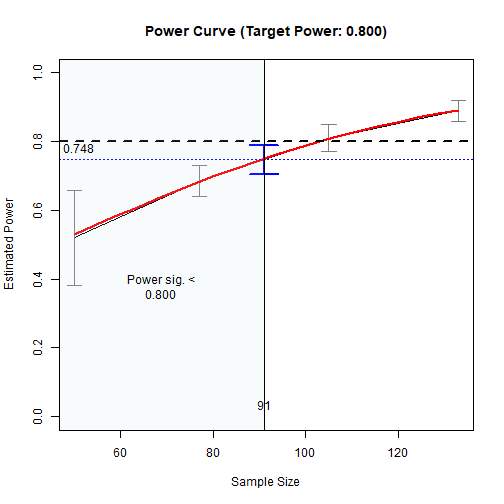

The Power Curve

The black line is the plot of the sample sizes studied, along with the estimated power levels and the 95% confidence intervals. The intervals may vary in width if the numbers of replications are not the same for the sample sizes examined.

The red line is the plot based on the model (a logistic model in this case), along the range of sample sizes examined.

The area to the left of the solution is the region for which the power is estimated to be significantly less than the target power.

Case 2

Let’s consider Case 2, finding the sample size with the 95% confidence interval of its power approximately above the target power. That is, the lower bound of the confidence interval is close enough to the target power.

This is the function call:

out_n_lb <- n_from_power(out,
                         target_power = .80,
                         final_nrep = 400,
                         what = "lb",
                         seed = 2345)

The only change is what, which is set to "lb" (lower bound).

The example above only needs a few attempts to arrive at the approximation.

This is the output:

out_n_lb
#> Call:
#> power4mome::x_from_power(object = out, x = "n", target_power = 0.8, 
#>     what = "lb", goal = "close_enough", final_nrep = 400, seed = 2345)
#> 
#>                           Setting
#> Predictor(x):         Sample Size
#> Parameter:                    N/A
#> goal:                close_enough
#> what:                          lb
#> algorithm:              bisection
#> Level of confidence:       95.00%
#> Target Power:               0.800
#> 
#> - Final Value of Sample Size (n): 114
#> 
#> - Final Estimated Power (CI): 0.845 [0.810, 0.880]
#> 
#> Call `summary()` for detailed results.

The estimated sample size is 114. The estimated power based on simulation is 0.845, with its confidence interval equal to [0.810, 0.790]. The upper bound, 0.810, is .02 within the target power (.80).

With 400 replications, it is estimated that sample sizes greater than 114 have power significantly greater than .80 and can be used if the target power is .80.

This a summary of the results:

summary(out_n_lb)
#> 
#> ====== x_from_power Results ======
#> 
#> Call:
#> power4mome::x_from_power(object = out, x = "n", target_power = 0.8, 
#>     what = "lb", goal = "close_enough", final_nrep = 400, seed = 2345)
#> 
#> Predictor (x): Sample Size 
#> 
#> - Target Power: 0.800 
#> - Goal: Find 'x' with estimated lower confidence bound close enough to
#>   the target power.
#> 
#> === Major Results ===
#> 
#> - Final Value (Sample Size): 114
#> 
#> - Final Estimated Power: 0.845 
#> - Confidence Interval: [0.810; 0.880]
#> - Level of confidence: 95.0%
#> - Based on 400 replications.
#> 
#> === Technical Information ===
#> 
#> - Algorithm: bisection 
#> - Tolerance for 'close enough': Within 0.02000 of 0.800 
#> - The range of values explored: 109 to 98 
#> - Time spent in the search: 2.619 mins 
#> - The final crude model for the power-predictor relation:
#> 
#> Model Type: Logistic Regression 
#> 
#> Call:
#> power_curve(object = by_x_1, formula = power_model, start = power_curve_start, 
#>     lower_bound = lower_bound, upper_bound = upper_bound, nls_args = nls_args, 
#>     nls_control = nls_control, verbose = progress)
#> 
#> Predictor: n (Sample Size)
#> 
#> Model:
#> 
#> Call:  stats::glm(formula = reject ~ x, family = "binomial", data = reject1)
#> 
#> Coefficients:
#> (Intercept)            x  
#>    -1.10411      0.02393  
#> 
#> Degrees of Freedom: 2449 Total (i.e. Null);  2448 Residual
#> Null Deviance:       2381 
#> Residual Deviance: 2254  AIC: 2258
#> 
#> - Detailed Results:
#> 
#> [test]: test_indirect: x->m->y 
#> [test_label]: Test 
#>     n   est   p.v reject r.cilo r.cihi
#> 1  50 0.167 1.000  0.520  0.382  0.658
#> 2  77 0.151 1.000  0.672  0.627  0.718
#> 3  98 0.147 1.000  0.775  0.734  0.816
#> 4 109 0.151 1.000  0.815  0.777  0.853
#> 5 114 0.151 1.000  0.845  0.810  0.880
#> 6 119 0.149 1.000  0.855  0.820  0.890
#> 7 161 0.150 1.000  0.935  0.911  0.959
#> Notes:
#> - n: The sample size in a trial.
#> - p.v: The proportion of valid replications.
#> - est: The mean of the estimates in a test across replications.
#> - reject: The proportion of 'significant' replications, that is, the
#>   rejection rate. If the null hypothesis is true, this is the Type I
#>   error rate. If the null hypothesis is false, this is the power.
#> - r.cilo,r.cihi: The confidence interval of the rejection rate, based
#>   on normal approximation.
#> - Refer to the tests for the meanings of other columns.

This is a plot of the search:

plot(out_n_lb)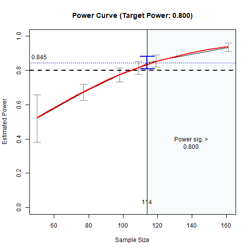

The Power Curve

Case 1, Case 2, or Both?

Similar to the Johnson-Neyman method in moderation, the two sample sizes found above can be used together to estimate the range of sample sizes with power not significantly different form the target power.

That is, from the results above, we can conclude that, with 400 replications, sample sizes from 91 to 114 have power levels not significantly different from .80.

However, we believe researchers rarely need to find “the” sample with exactly “the” target power and doing sample size planning.

Therefore, if resource is a concern and so it is more important not to have a sample size with power too low, then Case 1 is sufficient for knowing the range of sample sizes that should definitely not used.

If having sufficient power is more important and the associated resource is available, the Case 2 is appropriate because it can find the minimum sample size that will have power significantly higher than the target power.

Advanced Features

This brief illustration only covers basic features of n_from_power(). There are other ways to customize the search, such as the range of sample sizes to examine, the level of confidence for the confidence interval, and the number of trials (10 by default). Please refer to the help page of x_from_power(), which n_from_power() calls, for these and other options.

References

Cheung, S. F., & Cheung, S.-H. (2024). Manymome: An R package for computing the indirect effects, conditional effects, and conditional indirect effects, standardized or unstandardized, and their bootstrap confidence intervals, in many (though not all) models. Behavior Research Methods, 56(5), 4862–4882. https://doi.org/10.3758/s13428-023-02224-z

2025-08-31