Plot a Power Curve

Plotting the results in a 'power_curve' object, such as the estimated power against sample size, or the results of power4test_by_n() or power4test_by_es().

Usage

# S3 method for class 'power_curve'
plot(
  x,
  what = c("ci", "power_curve"),
  main = paste0("Power Curve ", "(Predictor: ", switch(x$predictor, n = "Sample Size", es
    = "Effect Size"), ")"),
  xlab = switch(x$predictor, n = "Sample Size", es = "Effect Size"),
  ylab = "Estimated Power",
  pars_ci = list(),
  type = "l",
  ylim = c(0, 1),
  ci_level = 0.95,
  ...
)

# S3 method for class 'power4test_by_n'
plot(
  x,
  what = c("ci", "power_curve"),
  main = "Estimated Power vs. Sample Size",
  xlab = "Sample Size",
  ylab = "Estimated Power",
  pars_ci = list(),
  type = "l",
  ylim = c(0, 1),
  ci_level = 0.95,
  ...
)

# S3 method for class 'power4test_by_es'
plot(
  x,
  what = c("ci", "power_curve"),
  main = paste0("Estimated Power vs. Effect Size / Parameter (", attr(x[[1]],
    "pop_es_name"), ")"),
  xlab = paste0("Effect Size / Parameter (", attr(x[[1]], "pop_es_name"), ")"),
  ylab = "Estiamted Power",
  pars_ci = list(),
  type = "l",
  ylim = c(0, 1),
  ci_level = 0.95,
  ...
)

Arguments

x

The object to be plotted. It can be a power_curve object, the output of power_curve(). It can also be the output of power4test_by_n() or power4test_by_es().

what

A character vector of what to include in the plot. Possible values are "ci" (confidence intervals for the estimated sample size) and "power_curve" (the crude power curve, if available). The default values depend on the type of x.

main

The title of the plot.

xlab, ylab

The labels for the horizontal and vertical axes, respectively.

pars_ci

A named list of arguments to be passed to arrows() to customize the drawing of the confidence intervals.

type

An argument of the default plot method plot.default(). Default is "l". See plot.default() for other options.

ylim

A two-element numeric vector of the range of the vertical axis.

ci_level

The level of confidence of the confidence intervals, if requested. Default is .95, denoting 95%.

...

Optional arguments. Passed to plot() when drawing the base plot.

Value

The plot-methods return x invisibly. They are called for their side effects.

Details

The plot method of power_curve objects currently plots the relation between estimated power and the predictor. Other elements can be requested (see the argument what), and they can be customized individually.

See also

power_curve(), power4test_by_n(), and power4test_by_es().

Examples

# Specify the population model

model_simple_med <-
"
m ~ x
y ~ m + x
"

# Specify the effect sizes (population parameter values)

model_simple_med_es <-
"
y ~ m: l
m ~ x: m
y ~ x: s
"

# Simulate datasets to check the model

sim_only <- power4test(nrep = 10,
                       model = model_simple_med,
                       pop_es = model_simple_med_es,
                       n = 50,
                       fit_model_args = list(fit_function = "lm"),
                       do_the_test = FALSE,
                       iseed = 1234,
                       parallel = FALSE,
                       progress = FALSE)

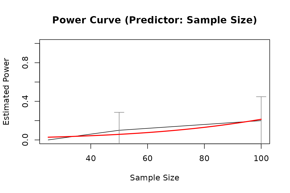
# By n: Do a test for different sample sizes
# Set `parallel` to TRUE for faster, usually much faster, analysis
# Set `progress` to TRUE to display the progress of the analysis

out1 <- power4test_by_n(sim_only,
                        nrep = 10,
                        test_fun = test_parameters,
                        test_args = list(par = "y~x"),
                        n = c(25, 50, 100),
                        by_seed = 1234,
                        parallel = FALSE,
                        progress = FALSE)

pout1 <- power_curve(out1)
pout1
#> Call:
#> power_curve(object = out1)
#> 
#> Predictor: n (Sample Size)
#> 
#> Model:
#> 
#> Call:  stats::glm(formula = reject ~ x, family = "binomial", data = reject1)
#> 
#> Coefficients:
#> (Intercept)            x  
#>    -4.28606      0.02986  
#> 
#> Degrees of Freedom: 29 Total (i.e. Null);  28 Residual
#> Null Deviance:	    19.5 
#> Residual Deviance: 17.37 	AIC: 21.37
plot(pout1)


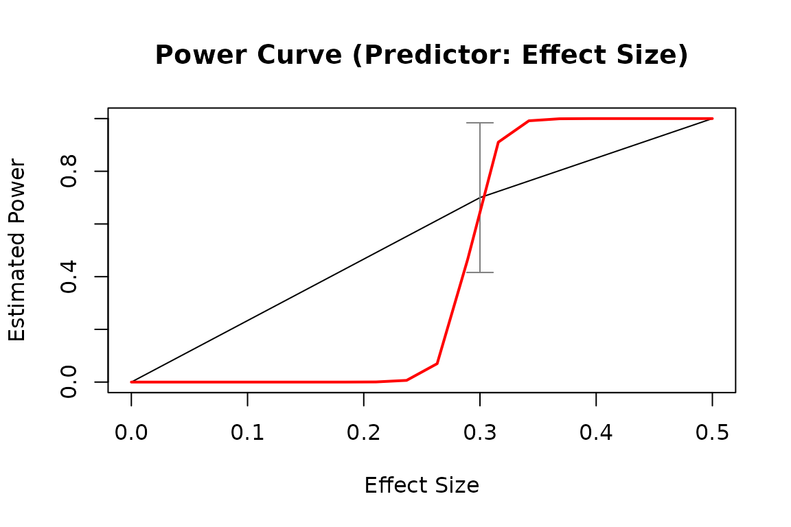
# By pop_es: Do a test for different population values of a model parameter
# Set `parallel` to TRUE for faster, usually much faster, analysis
# Set `progress` to TRUE to display the progress of the analysis

out2 <- power4test_by_es(sim_only,
                             nrep = 10,
                             test_fun = test_parameters,
                             test_args = list(par = "y~x"),
                             pop_es_name = "y ~ x",
                             pop_es_values = c(0, .3, .5),
                             by_seed = 1234,
                             parallel = FALSE,
                             progress = FALSE)

pout2 <- power_curve(out2)
plot(pout2)