Power Curve

Estimate the relation between power and a characteristic, such as sample size or population effect size (population value of a model parameter).

Usage

power_curve(
  object,
  formula = NULL,
  start = NULL,
  lower_bound = NULL,
  upper_bound = NULL,
  nls_args = list(),
  nls_control = list(),
  verbose = FALSE,
  models = c("nls", "logistic", "lm")
)

# S3 method for class 'power_curve'
print(x, data_used = FALSE, digits = 3, right = FALSE, row.names = FALSE, ...)

Arguments

object: An object of the class power4test_by_n or power4test_by_es, which is the output of power4test_by_n() or power4test_by_es().
formula: A formula of the model for stats::nls(). It can also be a list of formulas, and the models will be fitted successively by stats::nls(), with the first model fitted successfully adopted. The response variable in the formula must be named reject, and the predictor named x. Whether x represents n or es depends on the class of object. If NULL, the default, it will be determined internally based on the type of object.
start: Either a named vector of the start value(s) of parameter(s) in formula, or a list of named vectors of the starting value(s) of the list of formula(s). If NULL, the default, they will be determined internally.
lower_bound: Either a named vector of the lower bound(s) of parameter(s) in formula, or a list of named vectors of the lower bound(s) for the list of formula(s). They will be passed to lower of stats::nls(). If NULL, the default, it will be determined internally based on the type of object.
upper_bound: Either a named vector of the upper bound(s) of parameter(s) in formula, or a list of named vectors of the upper bound(s) for the list of formula(s). They will be passed to upper of stats::nls(). If NULL, the default, it will be determined internally based on the type of object.
nls_args: A named list of arguments to be used when calling stats::nls(). Used to override internal default, such as the algorithm (default is "port"). Use this argument with cautions.
nls_control: A named list of arguments to be passed the control argument of stats::nls(). The values will override internal default values, and also override nls_args. Use this argument with cautions.
verbose: Logical. Whether messages will be printed when trying different models.
models: Models to try. Support "nls" (fitted by nls()), "logistic" (fitted by glm()), and "lm" (fitted by lm()). By default, all three models will be attempted, in this order.
x: A power_curve object.
data_used: Logical. Whether the rejection rates data frame used to fit the model is printed.
digits, right, row.names: Arguments of the same names used by the print method of a data.frame object. Used when data_used is TRUE and the rejection rates data frame is printed.
...: For the print method of power_curve objects, they are optional arguments to be passed to print.data.frame() when printing the rejection rates data frame.

Value

It returns a list which is a power_curve object, with the following elements:

fit: The model fitted, which is the output of stats::nls(), stats::glm(), or stats::lm().
reject_df: The table of reject rates and other characteristics, which is generated by rejection_rates().
predictor: The predictor or the power curve, ether "n" (sample size) or "es" (population effect size).
call: The call used to run this function.

The print method of power_curve object returns x invisibly. Called for its side-effect.

Details

The function power_curve() retrieves the information from the output of power4test_by_n() or power4test_by_es(), and estimate the power curve: the relation between the characteristic varied, sample size for power4test_by_n() and the population effect size for power4test_by_es(), and the rejection rate of the test conducted by power4test_by_n() or power4test_by_es(). This rejection rate is the power when the null hypothesis is false (e.g., the population value of the effect size being tested is nonzero).

The model fitted is not intended to be a precise model for the relation across a wide range. It is only a crude estimate based on the limited number of values of the characteristic (e.g., sample size) examined, which can be as small as four or even smaller. The model is intended to be used for only for the range covered, and for estimating the probable sample size or effect size with a desirable level of power. This value should then be studied by higher precision through simulation using functions such as power4test().

These are the models to be tried, in the following order:

One or nonlinear models, to be fitted by stats::nls(). If several models are specified, all will be fitted and the one with the smallest deviance will be used.
If all the nonlinear models failed, for whatever reason, a logistic regression will be fitted by stats::glm() to predict the binary significant test results.
If the logistic model also failed, for whatever reason, a simple linear regression model will be fitted. Although the power curve is nonlinear across a wide range of, say, sample size, a linear model can still be a good enough approximation for a narrow range of the predictor.

The output can then be plotted to visualize the power curve, using the plot method (plot.power_curve()) for the output of power_curve().

This function can be used directly, but is also used internally by functions such as x_from_power().

Examples


# Specify the population model

model_simple_med <-
"
m ~ x
y ~ m + x
"

# Specify the effect sizes (population parameter values)

model_simple_med_es <-
"
y ~ m: l
m ~ x: m
y ~ x: s
"

# Simulate datasets to check the model
# Set `parallel` to TRUE for faster, usually much faster, analysis
# Set `progress` to TRUE to display the progress of the analysis

sim_only <- power4test(nrep = 10,
                       model = model_simple_med,
                       pop_es = model_simple_med_es,
                       n = 50,
                       fit_model_args = list(fit_function = "lm"),
                       do_the_test = FALSE,
                       iseed = 1234,
                       parallel = FALSE,
                       progress = FALSE)

# By n: Do a test for different sample sizes

out1 <- power4test_by_n(sim_only,
                        nrep = 10,
                        test_fun = test_parameters,
                        test_args = list(par = "y~x"),
                        n = c(25, 50, 100),
                        by_seed = 1234,
                        parallel = FALSE,
                        progress = FALSE)

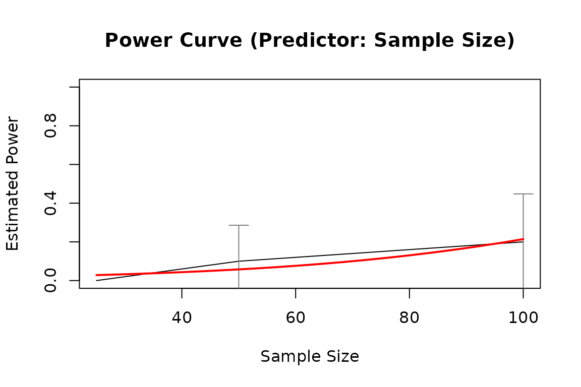
pout1 <- power_curve(out1)
pout1
#> Call:
#> power_curve(object = out1)
#> 
#> Predictor: n (Sample Size)
#> 
#> Model:
#> 
#> Call:  stats::glm(formula = reject ~ x, family = "binomial", data = reject1)
#> 
#> Coefficients:
#> (Intercept)            x  
#>    -4.28606      0.02986  
#> 
#> Degrees of Freedom: 29 Total (i.e. Null);  28 Residual
#> Null Deviance:	    19.5 
#> Residual Deviance: 17.37 	AIC: 21.37
plot(pout1)


# By pop_es: Do a test for different population values of a model parameter

out2 <- power4test_by_es(sim_only,
                         nrep = 10,
                         test_fun = test_parameters,
                         test_args = list(par = "y~x"),
                         pop_es_name = "y ~ x",
                         pop_es_values = c(0, .3, .5),
                         by_seed = 1234,
                         parallel = FALSE,
                         progress = FALSE)

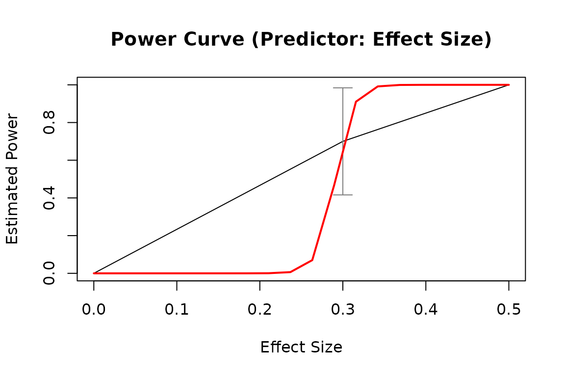
pout2 <- power_curve(out2)
pout2
#> Call:
#> power_curve(object = out2)
#> 
#> Predictor: es (Effect Size)
#> 
#> Model:
#> 
#> Call:  stats::glm(formula = reject ~ x, family = "binomial", data = reject1)
#> 
#> Coefficients:
#> (Intercept)            x  
#>      -27.13        93.25  
#> 
#> Degrees of Freedom: 29 Total (i.e. Null);  28 Residual
#> Null Deviance:	    41.05 
#> Residual Deviance: 12.22 	AIC: 16.22
plot(pout2)

Usage

Arguments

Value

Details

See also

Examples