Plot The Results of 'x_from_power'

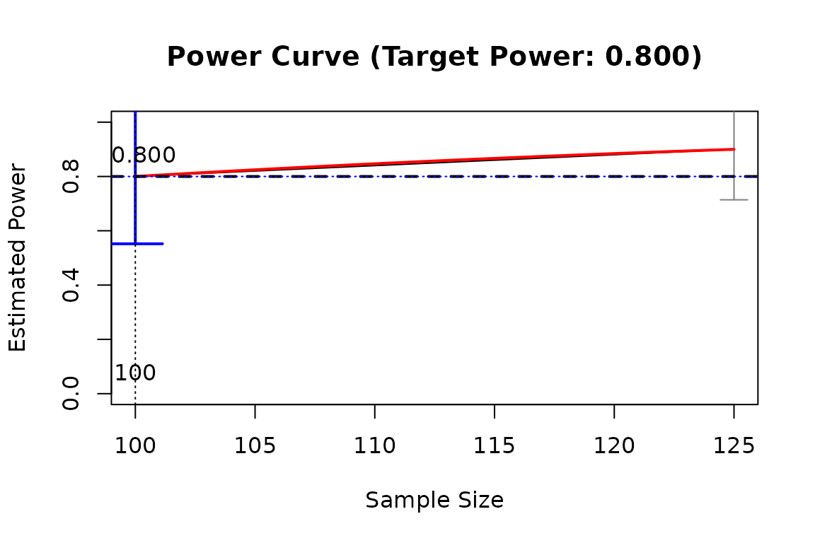
It plots the results of 'x_from_power', such as the estimated power against sample size.

Usage

# S3 method for class 'x_from_power'
plot(
  x,
  what = c("ci", "power_curve", "final_x", "final_power", "target_power", switch(x$x, n =
    "sig_area", es = NULL)),
  text_what = c("final_x", "final_power", switch(x$x, n = "sig_area", es = NULL)),
  digits = 3,
  main = paste0("Power Curve ", "(Target Power: ", formatC(x$target_power, digits =
    digits, format = "f"), ")"),
  xlab = NULL,
  ylab = "Estimated Power",
  ci_level = 0.95,
  pars_ci = list(),
  pars_power_curve = list(),
  pars_ci_final_x = list(lwd = 2, length = 0.2, col = "blue"),
  pars_target_power = list(lty = "dashed", lwd = 2, col = "black"),
  pars_final_x = list(lty = "dotted"),
  pars_final_power = list(lty = "dotted", col = "blue"),
  pars_text_final_x = list(y = 0, pos = 3, cex = 1),
  pars_text_final_power = list(pos = 3, cex = 1),
  pars_sig_area = list(col = adjustcolor("lightblue", alpha.f = 0.1)),
  pars_text_sig_area = list(cex = 1),
  ...
)

# S3 method for class 'n_region_from_power'
plot(
  x,
  what = c("ci", "power_curve", "final_x", "final_power", "target_power", "sig_area"),
  text_what = c("final_x", "final_power", "sig_area"),
  digits = 3,
  main = paste0("Power Curve ", "(Target Power: ", formatC(x$below$target_power, digits =
    digits, format = "f"), ")"),
  xlab = NULL,
  ylab = "Estimated Power",
  ci_level = 0.95,
  pars_ci = list(),
  pars_power_curve = list(),
  pars_ci_final_x = list(lwd = 2, length = 0.2, col = "blue"),
  pars_target_power = list(lty = "dashed", lwd = 2, col = "black"),
  pars_final_x = list(lty = "dotted"),
  pars_final_power = list(lty = "dotted", col = "blue"),
  pars_text_final_x = list(y = 0, pos = 3, cex = 1),
  pars_text_final_power = list(cex = 1),
  pars_sig_area = list(col = adjustcolor("lightblue", alpha.f = 0.1)),
  pars_text_sig_area = list(cex = 1),
  ...
)

Arguments

x: An x_from_power object, the output of x_from_power().
what: A character vector of what to include in the plot. Possible values are "ci" (confidence intervals for the estimated value of the predictor), "power_curve" (the crude power curve, if available), "final_x" (a vertical line for the value of the predictor with estimated power close enough to the target power by confidence interval), "final_power" (a horizontal line for the estimated power of the final value of the predictor), "target_power" (a horizontal line for the target power), and "sig_area" (the area significantly higher or lower than the target power, if goal is "close_enough" and what is "lb" or "ub"). By default, all these elements will be plotted.
text_what: A character vector of what numbers to be added as labels. Possible values are "final_x" (the value of the predictor with estimated power close enough to the target power by confidence interval) "final_power" (the estimated power of the final value of the predictor), and "sig_area" (labeling the area significantly higher or lower than the target power, if goal is "close_enough" and what is "lb" or "ub"). By default, all these labels will be added.
digits: The number of digits after the decimal that will be used when adding numbers.
main: The title of the plot.
xlab, ylab: The labels for the horizontal and vertical axes, respectively.
ci_level: The level of confidence of the confidence intervals, if requested. Default is .95, denoting 95%.
pars_ci: A named list of arguments to be passed to arrows() to customize the drawing of the confidence intervals.
pars_power_curve: A named list of arguments to be passed to points() to customize the drawing of the power curve.
pars_ci_final_x: A named list of arguments to be passed to arrows() to customize the drawing of the confidence interval of the final value of the predictor.
pars_target_power: A named list of arguments to be passed to abline() when drawing the horizontal line for the target power.
pars_final_x: A named list of arguments to be passed to abline() when drawing the vertical line for the final value of the predictor.
pars_final_power: A named list of arguments to be passed to abline() when drawing the horizontal line for the estimated power at the final value of the predictor.
pars_text_final_x: A named list of arguments to be passed to text() when adding the label for the final value of the predictor.
pars_text_final_power: A named list of arguments to be passed to text() when adding the label for the estimated power of final value of the predictor.
pars_sig_area: A named list of arguments to be passed to rect() when shading the area significantly higher or lower than the target power.
pars_text_sig_area: A named list of arguments to be passed to text() when labelling the area significantly higher or lower than the target power.
...: Optional arguments. Passed to plot() when drawing the estimated power against the predictor.

Value

The plot-method of x_from_power returns x invisibly. It is called for its side effect.

The plot-method of n_region_from_power returns x invisibly. It is called for its side effect.

Details

The plot method of x_from_power objects currently plots the relation between estimated power and the values examined by x_from_power(). Other elements can be requested (see the argument what), and they can be customized individually.

The plot-method for n_region_from_power objects is a modified version of the plot-method for x_from_power. It plots the results of two runs of n_from_power() in one plot. It is otherwise similar to the plot-method for x_from_power.

Examples


# Specify the population model

mod <-
"
m ~ x
y ~ m + x
"

# Specify the population values

mod_es <-
"
m ~ x: m
y ~ m: l
y ~ x: n
"

# Generate the datasets

sim_only <- power4test(nrep = 10,
                       model = mod,
                       pop_es = mod_es,
                       n = 100,
                       do_the_test = FALSE,
                       iseed = 1234)
#> Simulate the data:
#> Fit the model(s):

# Do a test

test_out <- power4test(object = sim_only,
                       test_fun = test_parameters,
                       test_args = list(pars = "m~x"))
#> Do the test: test_parameters: CIs (pars: m~x) 

# Determine the sample size with a power of .80 (default)

power_vs_n <- x_from_power(test_out,
                           x = "n",
                           progress = TRUE,
                           target_power = .80,
                           final_nrep = 10,
                           max_trials = 1,
                           seed = 2345)
#> 
#> --- Setting ---
#> 
#> Algorithm:  bisection 
#> Goal:  ci_hit 
#> What:  point   (Estimated Power) 
#> 
#> --- Progress  ---
#> 
#> - Set 'progress = FALSE' to suppress displaying the progress.
#> - Set 'simulation progress = FALSE' to suppress displaying the progress
#>   in the simulation.
#> 
#> Initial interval: [100, 125] 
#> 
#> 
#> Do the simulation for the upper bound:
#> 
#> Try x = 125 
#> 
#> Updating the simulation for sample size: 125 
#> Re-simulate the data:
#> Fit the model(s):
#> Update the test(s):
#> Update test_parameters: CIs (pars: m~x) :
#> 
#> Estimated power at n: 0.900, 95.0% confidence interval: [0.714,1.086]
#> 
#> Initial interval: [100, 125] 
#> 
#> - Rejection Rates:
#> [test]: test_parameters: CIs (pars: m~x) 
#> [test_label]: m~x 
#>     n   est   p.v reject r.cilo r.cihi
#> 1 100 0.320 1.000  0.800  0.552  1.048
#> 2 125 0.314 1.000  0.900  0.714  1.086
#> 
#> One of the bounds in the interval is already a solution.
#> 
#> - 'nls()' estimation skipped when less than 4 values of predictor examined.
#> Solution found.
#> 
#> 
#> --- Final Stage ---
#> 
#> - Start at 2025-09-05 00:16:10 
#> - Rejection Rates:
#> 
#> [test]: test_parameters: CIs (pars: m~x) 
#> [test_label]: m~x 
#>     n   est   p.v reject r.cilo r.cihi
#> 1 100 0.320 1.000  0.800  0.552  1.048
#> 2 125 0.314 1.000  0.900  0.714  1.086
#> Notes:
#> - n: The sample size in a trial.
#> - p.v: The proportion of valid replications.
#> - est: The mean of the estimates in a test across replications.
#> - reject: The proportion of 'significant' replications, that is, the
#>   rejection rate. If the null hypothesis is true, this is the Type I
#>   error rate. If the null hypothesis is false, this is the power.
#> - r.cilo,r.cihi: The confidence interval of the rejection rate, based
#>   on normal approximation.
#> - Refer to the tests for the meanings of other columns.
#> 
#> - Estimated Power Curve:
#> 
#> Call:
#> power_curve(object = by_x_1, formula = power_model, start = power_curve_start, 
#>     lower_bound = lower_bound, upper_bound = upper_bound, nls_args = nls_args, 
#>     nls_control = nls_control, verbose = progress)
#> 
#> Predictor: n (Sample Size)
#> 
#> Model:
#> 
#> Call:  stats::glm(formula = reject ~ x, family = "binomial", data = reject1)
#> 
#> Coefficients:
#> (Intercept)            x  
#>    -1.85743      0.03244  
#> 
#> Degrees of Freedom: 19 Total (i.e. Null);  18 Residual
#> Null Deviance:	    16.91 
#> Residual Deviance: 16.51 	AIC: 20.51
#> 
#> 
#> - Final Value: 100 
#> 
#> - Final Estimated Power: 0.8000 
#> - Confidence Interval: [0.5521; 1.0479]
#> - CI Level: 95.00%
plot(power_vs_n)

Usage

Arguments

Value

Details

See also

Examples