Quick Start To set_sem_layout

Introduction

The package semptools (CRAN page) contains functions that post-process an output from semPlot::semPaths(), to help users to customize the appearance of the graphs generated by semPlot::semPaths(). For the introduction to functions for doing very specific tasks, such as moving the parameter estimate of a path or rotating the residual of a variable, please refer to vignette("semptools"). The present guide focuses on how to use set_sem_layout() to configure various aspects of a semPaths graph generated for a typical structural equation model (SEM) with latent factors. For configuring the layout of a confirmatory factor analysis (CFA) model with no structural path between factors, please refer to the vignette("quick_start_cfa").

The Initial `semPaths` Graph

Let us consider an SEM model. We will use sem_example, a sample CFA dataset from semptools with 14 variables for illustration.

library(semptools)
head(round(sem_example, 3), 3)
#>      x01    x02    x03    x04    x05    x06    x07    x08    x09    x10   x11
#> 1  2.861  2.289  3.381  0.191  0.095 -0.395 -0.060  1.320  2.807  2.330 2.069
#> 2 -0.246 -1.299 -0.371  2.232 -0.419 -0.565 -0.162  3.050  1.513  1.777 2.991
#> 3  0.079  0.067  0.323 -3.043 -1.093 -0.626 -1.961 -4.908 -2.048 -3.190 1.403
#>     x12    x13   x14
#> 1 0.569 -0.808 1.989
#> 2 2.125  0.767 1.539
#> 3 1.888  1.356 1.107

This is the SEM model to be fitted:

mod <-
  'f1 =~ x01 + x02 + x03
   f2 =~ x04 + x05 + x06 + x07
   f3 =~ x08 + x09 + x10
   f4 =~ x11 + x12 + x13 + x14
   f3 ~  f1 + f2
   f4 ~  f1 + f3
  '

Fitting the model using lavaan::sem():

library(lavaan)
#> This is lavaan 0.6-19
#> lavaan is FREE software! Please report any bugs.
fit <- lavaan::sem(mod, cfa_example)

This is the plot from semPaths:

library(semPlot)
p <- semPaths(fit, whatLabels="est",
        sizeMan = 5,
        node.width = 1,
        edge.label.cex = .75,
        style = "ram",
        mar = c(5, 5, 5, 5))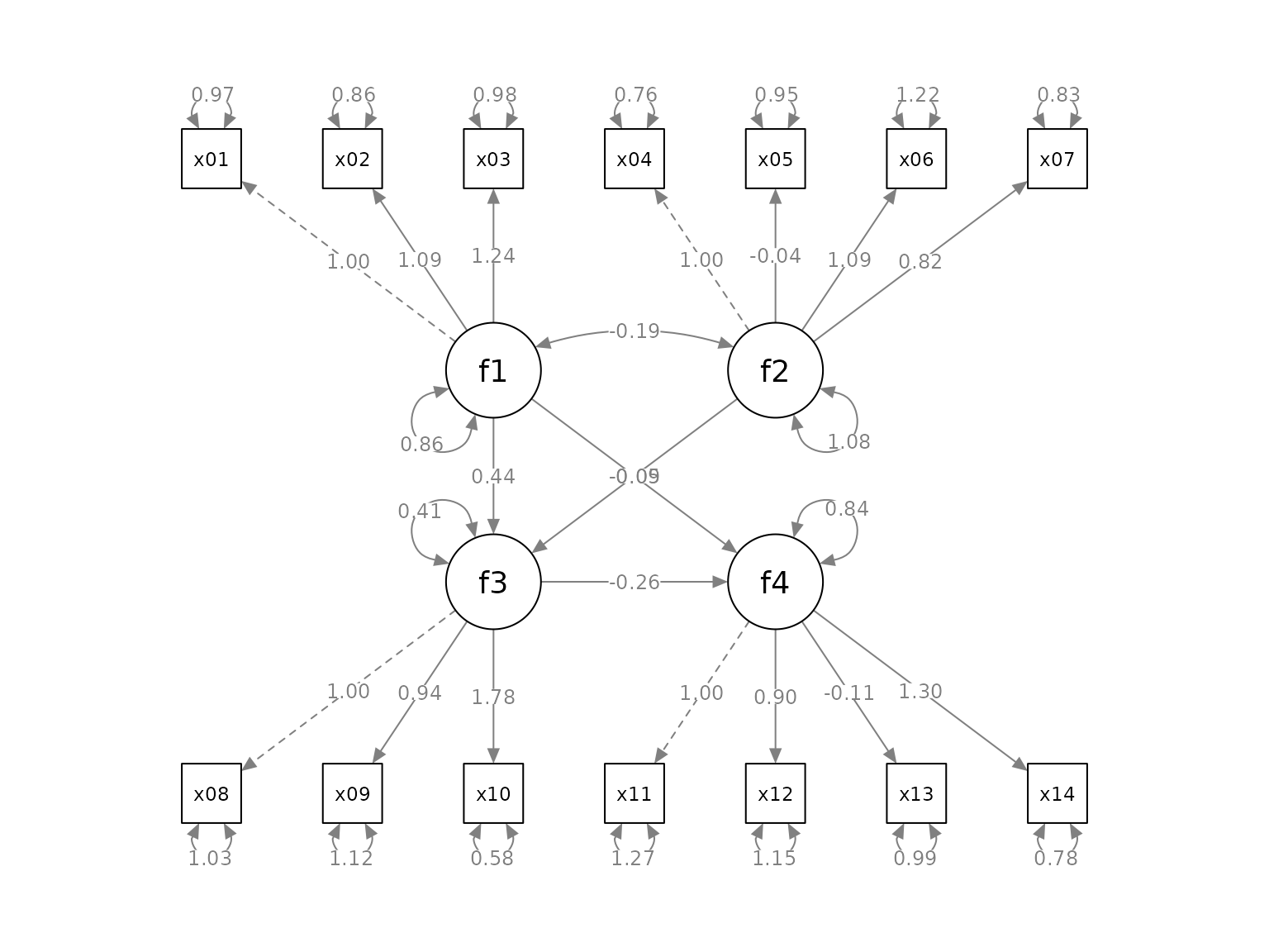

We will see how set_sem_layout() can be used to do the following tasks to post-process the graph:

Change the order of the indicators.
Assign factors to indicators manually.
Specify how to set the approximate positions of the factors.
Specify how to place the indicators of a factor.
Adjust the placement of the indicators relative to their corresponding factors.
Move the loadings along the paths from factors to indicators.

Assign Indicators to Factors

This section describes how to set the order of the indicators, assign them to factors, and specify the approximate positions of the factors.

Suppose we want to do this:

We would like to assign the indicators to the factors this way:
- x04, x05, x06, and x07 for f2.
- x01, x02, and x03 for f1.
- x11, x12, x13, and x14 for f4.
- x08, x09, and x10 for f3.

To do this, we create two vectors, one for the argument indicator_order and the other for the argument indicator_factor.

indicator_order is a string vector with length equal to the number of indicators, with the desired order if the indicators are placed above the corresponding factors. In this example, it will be like this:

indicator_order  <- c("x04", "x05", "x06", "x07",
                      "x01", "x02", "x03",
                      "x11", "x12", "x13", "x14",
                      "x08", "x09", "x10")

indicator_factor is a string vector with length equal to the number of indicators. The elements are the names of the latent factors, denoting which factor each indicator will be assigned to:

indicator_factor <- c( "f2",  "f2",  "f2",  "f2",
                       "f1",  "f1",  "f1",
                       "f4",  "f4",  "f4",  "f4",
                       "f3",  "f3",  "f3")

To specify the locations of the factors, we need two more arguments, factor_layout and factor_point_to.

factor_layout is a matrix of arbitrary size, with either NA or the name of a factor. For example:

factor_layout <- matrix(c("f1",   NA,   NA,
                           NA, "f3", "f4",
                         "f2",   NA,   NA), byrow = TRUE, 3, 3)

This sets up a 3-by-3 grid, with f1 on the top left, f2 on the bottom left, f3 in the center, and f4 on the right of f3. Each factor must be in one and only one cell of this matrix.

Note that a column or row can contain only NA, to increase the vertical or horizontal distance between factors.

The helper function layout_matrix() can also be used to create the matrix to be used in factor_layout (see vignette("layout_matrix") on how to use layout_matrix()):

factor_layout <- layout_matrix(f1 = c(1, 1),
                               f2 = c(3, 1),
                               f3 = c(2, 2),
                               f4 = c(2, 3))
factor_layout
#>      [,1] [,2] [,3]
#> [1,] "f1" NA   NA  
#> [2,] NA   "f3" "f4"
#> [3,] "f2" NA   NA

factor_point_to is a matrix of the size as factor_layout, with either NA or one of these: “down”, “left”, “up”, or “right”, to indicate the direction that a factor “points to” its indicator. For example:

factor_point_to <- matrix(c("left",     NA,      NA,
                                NA, "down", "down",
                            "left",     NA,      NA), byrow = TRUE, 3, 3)

f1 and f2 will point to the left (i.e., indicators on the left), f3 and f4 will point downwards.

layout_matrix() can also be used to create this matrix:

factor_point_to <- layout_matrix(left = c(1, 1),
                                 left = c(3, 1),
                                 down = c(2, 2),
                                 down = c(2, 3))
factor_point_to
#>      [,1]   [,2]   [,3]  
#> [1,] "left" NA     NA    
#> [2,] NA     "down" "down"
#> [3,] "left" NA     NA

In sum, the set_sem_layout() function needs at least these arguments:

semPaths_plot: The semPaths plot.
indicator_order: The vector for the order of indicators.
indicator_factor: The vector for assigning indicators to latent factors.
factor_layout: The position of the factors on a grid.
factor_point_to: The placement of the indicators.

They do not have to be named if they are in this order.

We now use set_sem_layout() to post-process the graph:

p2 <- set_sem_layout(p,
                     indicator_order = indicator_order,
                     indicator_factor = indicator_factor,
                     factor_layout = factor_layout,
                     factor_point_to = factor_point_to)
plot(p2)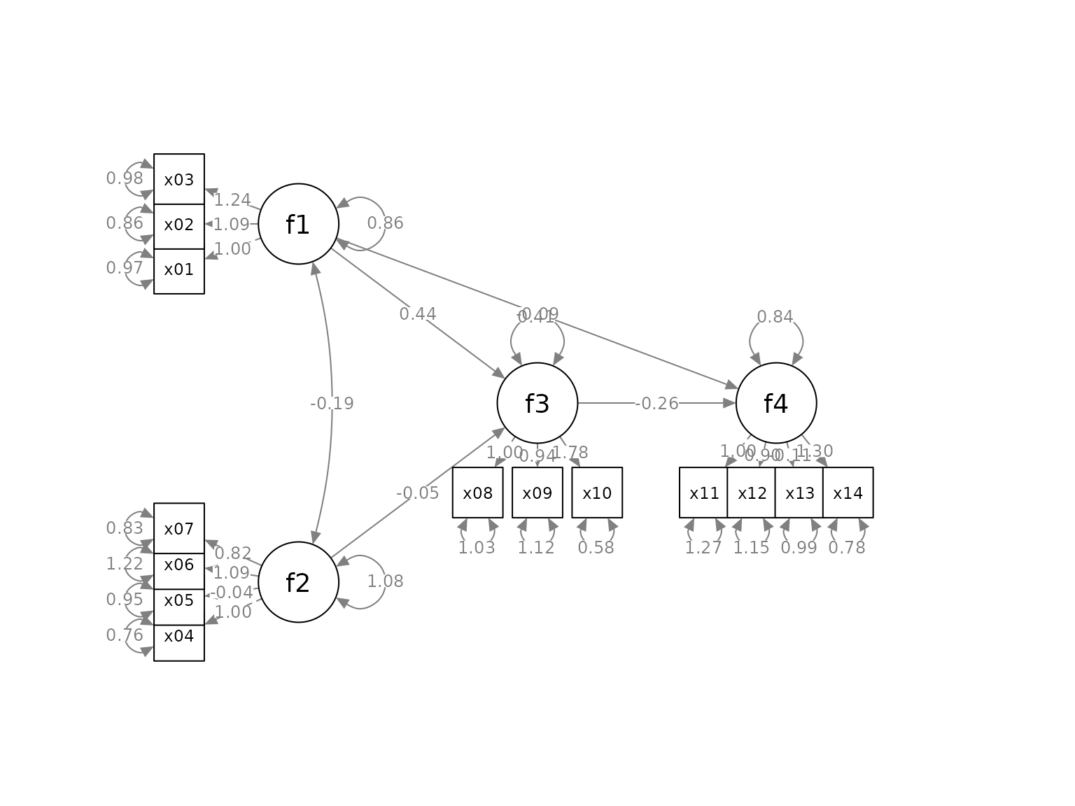

Move Indicators

The placement of the indicators are too close to the indicators and to neighboring indicators. We can adjust the relative position in two ways.

“Push” the indicators away

We can use the argument indicator_push to push the indicators of a factor away from it. The argument needs a named vector. The name is the factor of which the indictors will be “pushed”, and the value is how “hard” the push is: the multiplier to the distance from the factor to the indicators. For example:

indicator_push <- c(f3 = 2,
                    f4 = 1.5,
                    f1 = 1.5,
                    f2 = 1.5)

This vector will double the distance between the indicators of f3 and their factors, and multiply the distance between the indicators of f4, f1, and f2 and their factors by 1.5. If push is less than 1, the indicators will be “pulled” towards their factors.

p2 <- set_sem_layout(p,
                     indicator_order = indicator_order,
                     indicator_factor = indicator_factor,
                     factor_layout = factor_layout,
                     factor_point_to = factor_point_to,
                     indicator_push = indicator_push)
plot(p2)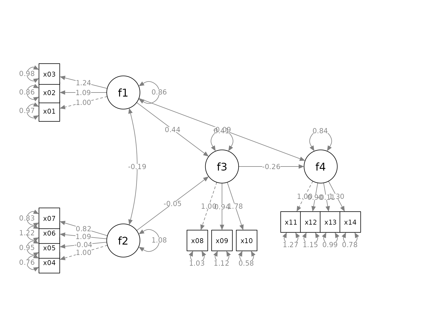

“Spread” out the indicators

We can use the argument indicator_spread to spread out the indicators of a factor, increasing the distance between the indicators. The argument needs a named vector. The name is the factor of which the indicators will be spread out. The value is the multiplier to the distance between neighboring indicators. For example:

indicator_spread <- c(f1 = 2,
                      f2 = 1.5,
                      f4 = 1.5)

This vector will double the distance between the indicators of f1, and multiply the distance between the indicators of f2 and f4. and its indicators by 1.5. If spread is less than 1, the indicators will be squeezed towards each others.

p2 <- set_sem_layout(p,
                     indicator_order = indicator_order,
                     indicator_factor = indicator_factor,
                     factor_layout = factor_layout,
                     factor_point_to = factor_point_to,
                     indicator_push = indicator_push,
                     indicator_spread = indicator_spread)
plot(p2)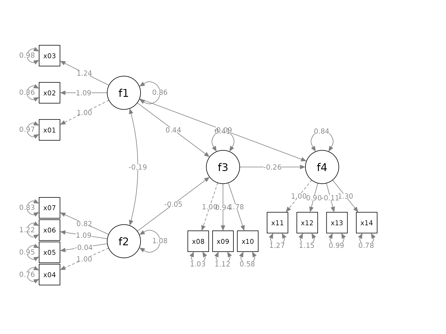

Move the Loadings

We can move the loadings of indicators along the paths by the argument loading_position. If we supply one single number, from 0 to 1, this number will be used for the position of all loadings. A value of .5 place the loadings on the middle of the paths. Larger the value, closer the loadings to the indicators. Smaller the value, closer the loadings to the factors.

We can also use a named vector to specify the positions of indicators for each factor.In each element, the name if the factor whose loadings will be moved. The value is the positions of its loadings. The default is .50. We only need to specify the positions for factors to be changed from .50 to other values. For example:

loading_position <- c(f2 = .7,
                      f3 = .8,
                      f4 = .8)

p2 <- set_sem_layout(p,
                     indicator_order = indicator_order,
                     indicator_factor = indicator_factor,
                     factor_layout = factor_layout,
                     factor_point_to = factor_point_to,
                     indicator_push = indicator_push,
                     indicator_spread = indicator_spread,
                     loading_position = loading_position)
plot(p2)

Pipe

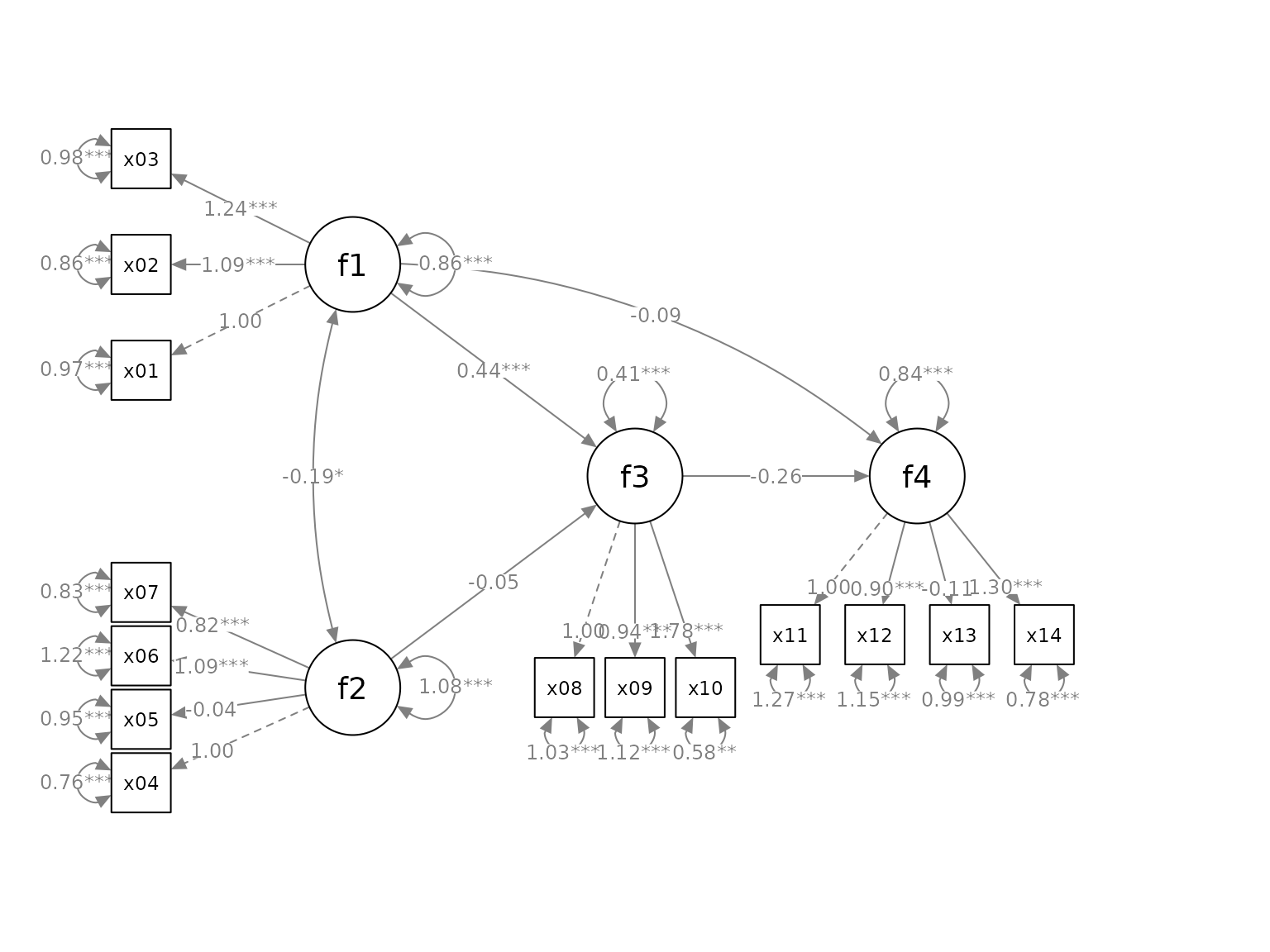
Like other functions in semptools, the set_sem_layout() function can be chained with other functions using the pipe operator, %>%, from the package magrittr, or the native pipe operator |> available since R 4.1.x. Suppose we want to mark the significant test results for the free parameters using mark_sig(), and use set_curve() to change the curvature of f1 ~~ f2 covariances and f4 ~ f1 paths (we push and spread some indicators to make room for the asterisks, and change the orientation of f4 to up):

# If R version >= 4.1.0
p2 <- set_sem_layout(p,
                    indicator_order = indicator_order,
                    indicator_factor = indicator_factor,
                    factor_layout = factor_layout,
                    factor_point_to = factor_point_to,
                    indicator_push = indicator_push,
                    indicator_spread = indicator_spread,
                    loading_position = loading_position) |>
                    set_curve(c("f2 ~~ f1" = -1,
                                "f4 ~ f1" = 1.5)) |>
                    mark_sig(fit)
plot(p2)

#> Loading required package: magrittr

Limitations

Currently, if a function needs the SEM output, only lavaan output is supported.

Shu Fai Cheung & Mark Hok Chio Lai

2024-12-17

Introduction

The Initial `semPaths` Graph

Assign Indicators to Factors

Move Indicators

“Push” the indicators away

“Spread” out the indicators

Move the Loadings

Pipe

Limitations

Quick Start To set_sem_layout

Shu Fai Cheung & Mark Hok Chio Lai

2024-12-17

Introduction

The Initial semPaths Graph

Assign Indicators to Factors

Move Indicators

“Push” the indicators away

“Spread” out the indicators

Move the Loadings

Pipe

Limitations

The Initial `semPaths` Graph