Mark parameter estimates (edge labels) based on p-value.
Usage
mark_sig(
  semPaths_plot,
  object = NULL,
  alphas = c(`*` = 0.05, `**` = 0.01, `***` = 0.001),
  ests = NULL,
  std_type = FALSE,
  ests_r2 = NULL,
  r2_prefix = "R2="
)
Arguments
- semPaths_plot
A qgraph::qgraph object generated by semPaths, or a similar qgraph object modified by other semptools functions.
- object
The object used by semPaths to generate the plot. Use the same argument name used in semPaths to make the meaning of this argument obvious. Currently only object of class
lavaanis supported.- alphas
A named numeric vector. Each element is the cutoff (level of significance), and the name of it is the symbol to be used if p-value is less than this cutoff. The default is c("" = .05, "" = .01, "" = .001).
- ests
A data.frame from the
parameterEstimatesfunction, or from other function with these columns:lhs,op,rhs, andpvalue. Only used whenobjectis not specified.- std_type
If standardized solution is used in the plot, set this either to the type of standardization (e.g.,
"std.all") or toTRUE. It will be passed tolavaan::standardizedSolution()to compute the p-values for the standardized solution. Used only if p-values are not supplied directly throughests.- ests_r2
A data.frame with these columns:
lhsandpvalue, storing the p-values for R-squares of the variables listed onlhs. If provided, the p-values in this data.frame will override those inobjectorests, if any. Used only when R-squares are present in thesemPaths_plot.- r2_prefix
The prefix used to identify R-squares in
semPaths_plot. Default is"R2=".
Value
A qgraph::qgraph based on the original one, with marks appended to edge labels based on their p-values.
Details
Modify a qgraph::qgraph object generated by semPaths and add marks (currently asterisk, "*") to the labels based on their p-values. Require either the original object used in the semPaths call, or a data frame with the p-values for each parameter. The latter option is for p-values not computed by lavaan but by other functions.
Currently supports only plots based on lavaan output.
R-squares
Normally, lavaan does not compute
p-values for R-squares. If
R-squares are detected in the plot
(based on r2_prefix), they will not
be marked, except for the following
conditions:
Users set
eststo a data frame with R-squares (op= "r2") as well as their p-values (underpvalue) computed by some methods.Users set
ests_r2to a data frame storing only the p-values for R-squares computed by some methods (and let the function find the p-values for other parameters fromobject).
Examples
mod_pa <-
'x1 ~~ x2
x3 ~ x1 + x2
x4 ~ x1 + x3
'
fit_pa <- lavaan::sem(mod_pa, pa_example)
lavaan::parameterEstimates(fit_pa)[, c("lhs", "op", "rhs", "est", "pvalue")]
#> lhs op rhs est pvalue
#> 1 x1 ~~ x2 0.005 0.957
#> 2 x3 ~ x1 0.537 0.000
#> 3 x3 ~ x2 0.376 0.000
#> 4 x4 ~ x1 0.111 0.382
#> 5 x4 ~ x3 0.629 0.000
#> 6 x3 ~~ x3 0.874 0.000
#> 7 x4 ~~ x4 1.194 0.000
#> 8 x1 ~~ x1 0.933 0.000
#> 9 x2 ~~ x2 1.017 0.000
m <- matrix(c("x1", NA, NA,
NA, "x3", "x4",
"x2", NA, NA), byrow = TRUE, 3, 3)
p_pa <- semPlot::semPaths(fit_pa, whatLabels="est",
style = "ram",
nCharNodes = 0, nCharEdges = 0,
layout = m)
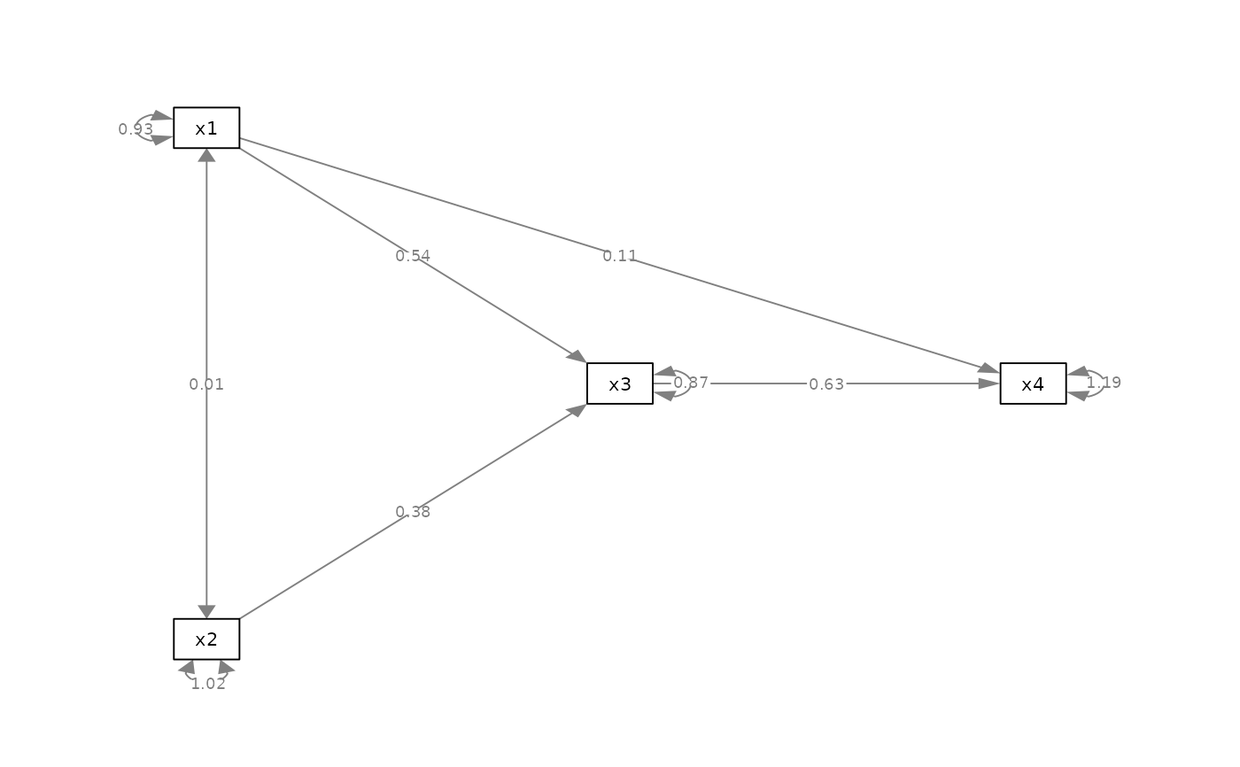 p_pa2 <- mark_sig(p_pa, fit_pa)
plot(p_pa2)
p_pa2 <- mark_sig(p_pa, fit_pa)
plot(p_pa2)
 mod_cfa <-
'f1 =~ x01 + x02 + x03
f2 =~ x04 + x05 + x06 + x07
f3 =~ x08 + x09 + x10
f4 =~ x11 + x12 + x13 + x14
'
fit_cfa <- lavaan::sem(mod_cfa, cfa_example)
lavaan::parameterEstimates(fit_cfa)[, c("lhs", "op", "rhs", "est", "pvalue")]
#> lhs op rhs est pvalue
#> 1 f1 =~ x01 1.000 NA
#> 2 f1 =~ x02 1.097 0.000
#> 3 f1 =~ x03 1.247 0.000
#> 4 f2 =~ x04 1.000 NA
#> 5 f2 =~ x05 -0.040 0.587
#> 6 f2 =~ x06 1.098 0.000
#> 7 f2 =~ x07 0.771 0.000
#> 8 f3 =~ x08 1.000 NA
#> 9 f3 =~ x09 0.937 0.000
#> 10 f3 =~ x10 1.785 0.000
#> 11 f4 =~ x11 1.000 NA
#> 12 f4 =~ x12 0.949 0.000
#> 13 f4 =~ x13 -0.077 0.356
#> 14 f4 =~ x14 1.184 0.000
#> 15 x01 ~~ x01 0.969 0.000
#> 16 x02 ~~ x02 0.853 0.000
#> 17 x03 ~~ x03 0.976 0.000
#> 18 x04 ~~ x04 0.725 0.000
#> 19 x05 ~~ x05 0.954 0.000
#> 20 x06 ~~ x06 1.161 0.000
#> 21 x07 ~~ x07 0.903 0.000
#> 22 x08 ~~ x08 1.026 0.000
#> 23 x09 ~~ x09 1.119 0.000
#> 24 x10 ~~ x10 0.566 0.009
#> 25 x11 ~~ x11 1.231 0.000
#> 26 x12 ~~ x12 1.032 0.000
#> 27 x13 ~~ x13 0.990 0.000
#> 28 x14 ~~ x14 0.985 0.000
#> 29 f1 ~~ f1 0.855 0.000
#> 30 f2 ~~ f2 1.119 0.000
#> 31 f3 ~~ f3 0.585 0.000
#> 32 f4 ~~ f4 0.943 0.000
#> 33 f1 ~~ f2 -0.173 0.059
#> 34 f1 ~~ f3 0.387 0.000
#> 35 f1 ~~ f4 -0.178 0.041
#> 36 f2 ~~ f3 -0.112 0.132
#> 37 f2 ~~ f4 0.593 0.000
#> 38 f3 ~~ f4 -0.181 0.014
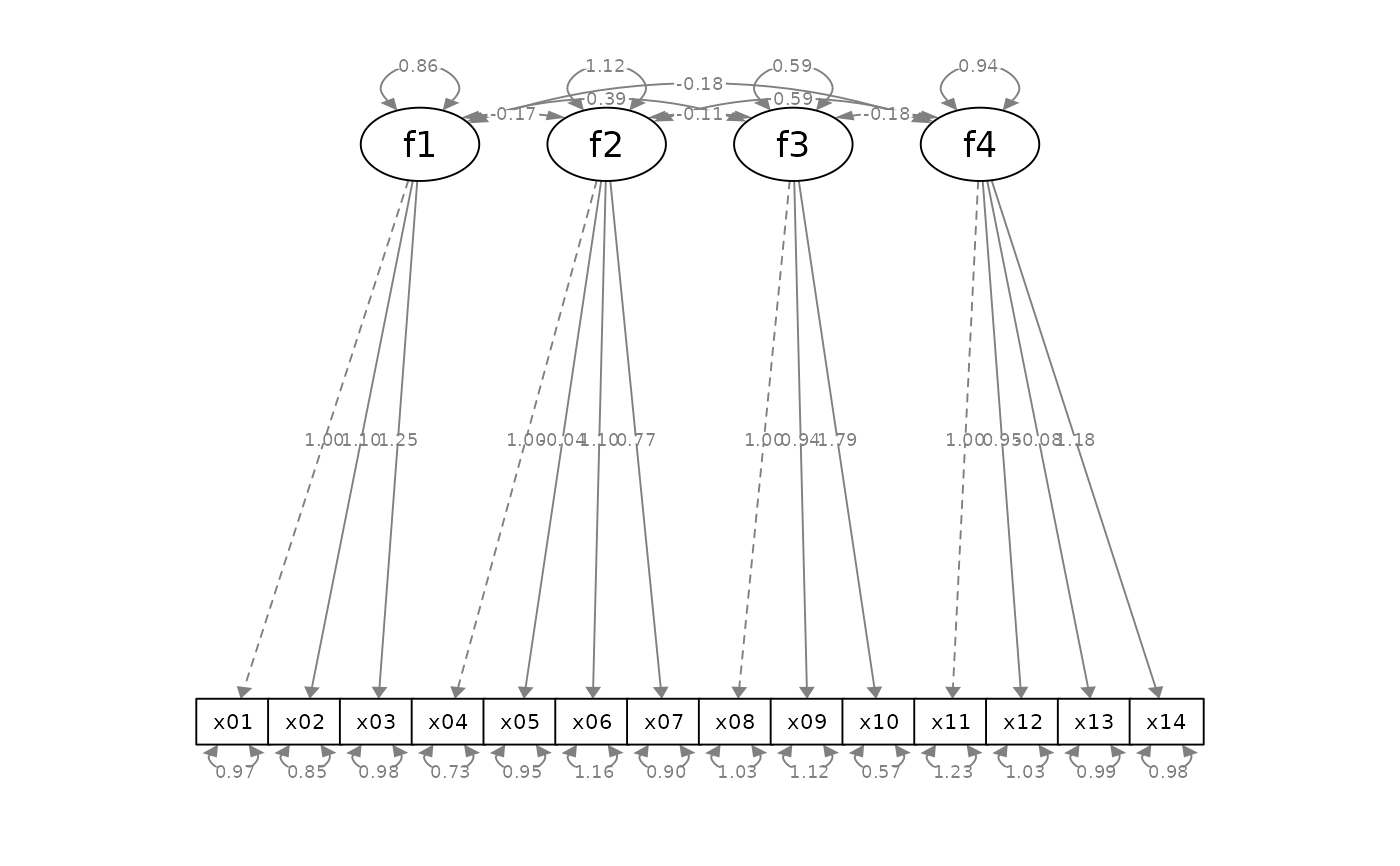
p_cfa <- semPlot::semPaths(fit_cfa, whatLabels="est",
style = "ram",
nCharNodes = 0, nCharEdges = 0)
mod_cfa <-
'f1 =~ x01 + x02 + x03
f2 =~ x04 + x05 + x06 + x07
f3 =~ x08 + x09 + x10
f4 =~ x11 + x12 + x13 + x14
'
fit_cfa <- lavaan::sem(mod_cfa, cfa_example)
lavaan::parameterEstimates(fit_cfa)[, c("lhs", "op", "rhs", "est", "pvalue")]
#> lhs op rhs est pvalue
#> 1 f1 =~ x01 1.000 NA
#> 2 f1 =~ x02 1.097 0.000
#> 3 f1 =~ x03 1.247 0.000
#> 4 f2 =~ x04 1.000 NA
#> 5 f2 =~ x05 -0.040 0.587
#> 6 f2 =~ x06 1.098 0.000
#> 7 f2 =~ x07 0.771 0.000
#> 8 f3 =~ x08 1.000 NA
#> 9 f3 =~ x09 0.937 0.000
#> 10 f3 =~ x10 1.785 0.000
#> 11 f4 =~ x11 1.000 NA
#> 12 f4 =~ x12 0.949 0.000
#> 13 f4 =~ x13 -0.077 0.356
#> 14 f4 =~ x14 1.184 0.000
#> 15 x01 ~~ x01 0.969 0.000
#> 16 x02 ~~ x02 0.853 0.000
#> 17 x03 ~~ x03 0.976 0.000
#> 18 x04 ~~ x04 0.725 0.000
#> 19 x05 ~~ x05 0.954 0.000
#> 20 x06 ~~ x06 1.161 0.000
#> 21 x07 ~~ x07 0.903 0.000
#> 22 x08 ~~ x08 1.026 0.000
#> 23 x09 ~~ x09 1.119 0.000
#> 24 x10 ~~ x10 0.566 0.009
#> 25 x11 ~~ x11 1.231 0.000
#> 26 x12 ~~ x12 1.032 0.000
#> 27 x13 ~~ x13 0.990 0.000
#> 28 x14 ~~ x14 0.985 0.000
#> 29 f1 ~~ f1 0.855 0.000
#> 30 f2 ~~ f2 1.119 0.000
#> 31 f3 ~~ f3 0.585 0.000
#> 32 f4 ~~ f4 0.943 0.000
#> 33 f1 ~~ f2 -0.173 0.059
#> 34 f1 ~~ f3 0.387 0.000
#> 35 f1 ~~ f4 -0.178 0.041
#> 36 f2 ~~ f3 -0.112 0.132
#> 37 f2 ~~ f4 0.593 0.000
#> 38 f3 ~~ f4 -0.181 0.014
p_cfa <- semPlot::semPaths(fit_cfa, whatLabels="est",
style = "ram",
nCharNodes = 0, nCharEdges = 0)
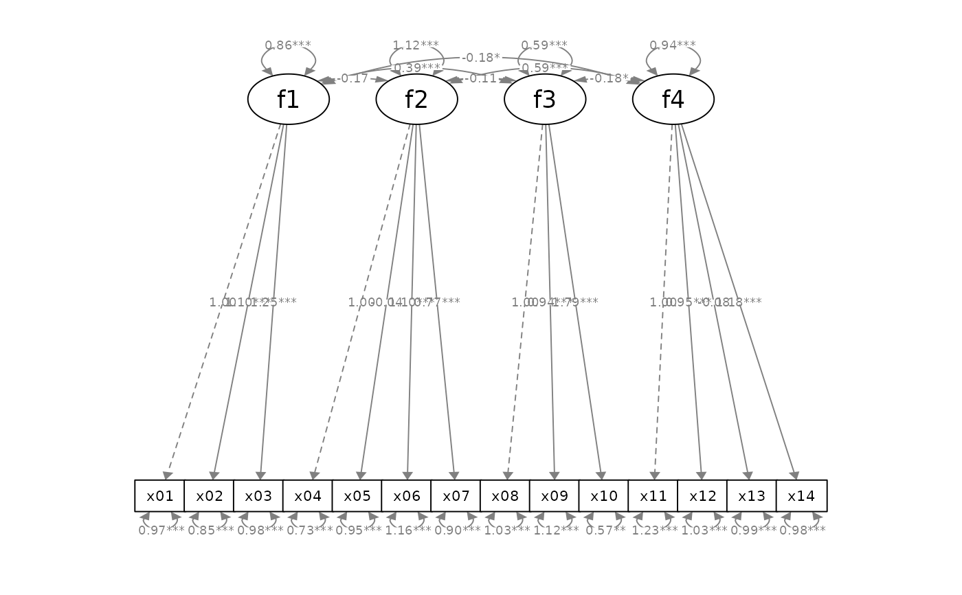
 p_cfa2 <- mark_sig(p_cfa, fit_cfa)
plot(p_cfa2)
p_cfa2 <- mark_sig(p_cfa, fit_cfa)
plot(p_cfa2)
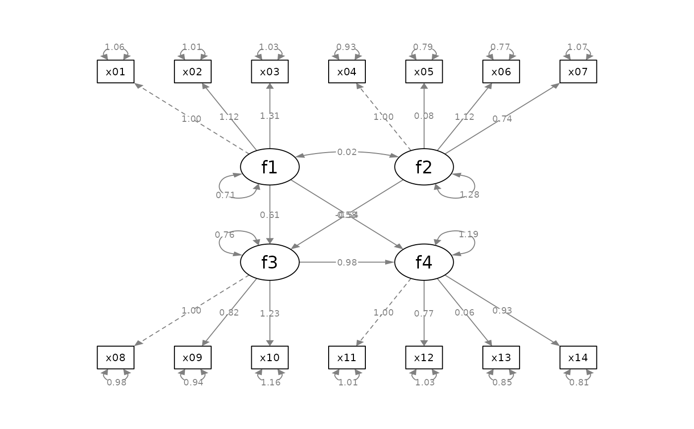
 mod_sem <-
'f1 =~ x01 + x02 + x03
f2 =~ x04 + x05 + x06 + x07
f3 =~ x08 + x09 + x10
f4 =~ x11 + x12 + x13 + x14
f3 ~ f1 + f2
f4 ~ f1 + f3
'
fit_sem <- lavaan::sem(mod_sem, sem_example)
lavaan::parameterEstimates(fit_sem)[, c("lhs", "op", "rhs", "est", "pvalue")]
#> lhs op rhs est pvalue
#> 1 f1 =~ x01 1.000 NA
#> 2 f1 =~ x02 1.124 0.000
#> 3 f1 =~ x03 1.310 0.000
#> 4 f2 =~ x04 1.000 NA
#> 5 f2 =~ x05 0.079 0.205
#> 6 f2 =~ x06 1.120 0.000
#> 7 f2 =~ x07 0.736 0.000
#> 8 f3 =~ x08 1.000 NA
#> 9 f3 =~ x09 0.819 0.000
#> 10 f3 =~ x10 1.230 0.000
#> 11 f4 =~ x11 1.000 NA
#> 12 f4 =~ x12 0.773 0.000
#> 13 f4 =~ x13 0.064 0.160
#> 14 f4 =~ x14 0.928 0.000
#> 15 f3 ~ f1 0.612 0.000
#> 16 f3 ~ f2 0.584 0.000
#> 17 f4 ~ f1 -0.542 0.001
#> 18 f4 ~ f3 0.980 0.000
#> 19 x01 ~~ x01 1.055 0.000
#> 20 x02 ~~ x02 1.015 0.000
#> 21 x03 ~~ x03 1.028 0.000
#> 22 x04 ~~ x04 0.933 0.000
#> 23 x05 ~~ x05 0.795 0.000
#> 24 x06 ~~ x06 0.771 0.000
#> 25 x07 ~~ x07 1.071 0.000
#> 26 x08 ~~ x08 0.976 0.000
#> 27 x09 ~~ x09 0.937 0.000
#> 28 x10 ~~ x10 1.164 0.000
#> 29 x11 ~~ x11 1.008 0.000
#> 30 x12 ~~ x12 1.033 0.000
#> 31 x13 ~~ x13 0.846 0.000
#> 32 x14 ~~ x14 0.807 0.000
#> 33 f1 ~~ f1 0.714 0.000
#> 34 f2 ~~ f2 1.277 0.000
#> 35 f3 ~~ f3 0.759 0.000
#> 36 f4 ~~ f4 1.188 0.000
#> 37 f1 ~~ f2 0.016 0.856
p_sem <- semPlot::semPaths(fit_sem, whatLabels="est",
style = "ram",
nCharNodes = 0, nCharEdges = 0)
mod_sem <-
'f1 =~ x01 + x02 + x03
f2 =~ x04 + x05 + x06 + x07
f3 =~ x08 + x09 + x10
f4 =~ x11 + x12 + x13 + x14
f3 ~ f1 + f2
f4 ~ f1 + f3
'
fit_sem <- lavaan::sem(mod_sem, sem_example)
lavaan::parameterEstimates(fit_sem)[, c("lhs", "op", "rhs", "est", "pvalue")]
#> lhs op rhs est pvalue
#> 1 f1 =~ x01 1.000 NA
#> 2 f1 =~ x02 1.124 0.000
#> 3 f1 =~ x03 1.310 0.000
#> 4 f2 =~ x04 1.000 NA
#> 5 f2 =~ x05 0.079 0.205
#> 6 f2 =~ x06 1.120 0.000
#> 7 f2 =~ x07 0.736 0.000
#> 8 f3 =~ x08 1.000 NA
#> 9 f3 =~ x09 0.819 0.000
#> 10 f3 =~ x10 1.230 0.000
#> 11 f4 =~ x11 1.000 NA
#> 12 f4 =~ x12 0.773 0.000
#> 13 f4 =~ x13 0.064 0.160
#> 14 f4 =~ x14 0.928 0.000
#> 15 f3 ~ f1 0.612 0.000
#> 16 f3 ~ f2 0.584 0.000
#> 17 f4 ~ f1 -0.542 0.001
#> 18 f4 ~ f3 0.980 0.000
#> 19 x01 ~~ x01 1.055 0.000
#> 20 x02 ~~ x02 1.015 0.000
#> 21 x03 ~~ x03 1.028 0.000
#> 22 x04 ~~ x04 0.933 0.000
#> 23 x05 ~~ x05 0.795 0.000
#> 24 x06 ~~ x06 0.771 0.000
#> 25 x07 ~~ x07 1.071 0.000
#> 26 x08 ~~ x08 0.976 0.000
#> 27 x09 ~~ x09 0.937 0.000
#> 28 x10 ~~ x10 1.164 0.000
#> 29 x11 ~~ x11 1.008 0.000
#> 30 x12 ~~ x12 1.033 0.000
#> 31 x13 ~~ x13 0.846 0.000
#> 32 x14 ~~ x14 0.807 0.000
#> 33 f1 ~~ f1 0.714 0.000
#> 34 f2 ~~ f2 1.277 0.000
#> 35 f3 ~~ f3 0.759 0.000
#> 36 f4 ~~ f4 1.188 0.000
#> 37 f1 ~~ f2 0.016 0.856
p_sem <- semPlot::semPaths(fit_sem, whatLabels="est",
style = "ram",
nCharNodes = 0, nCharEdges = 0)
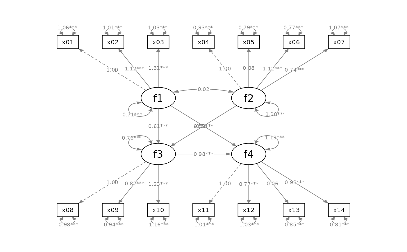
 p_sem2 <- mark_sig(p_sem, fit_sem)
plot(p_sem2)
p_sem2 <- mark_sig(p_sem, fit_sem)
plot(p_sem2)