Add Standard Error/Confidence Interval Estimates to Parameter Estimates (Edge Labels)
Source:R/mark_se.R
mark_se.RdAdd standard error or confidence interval estimates, in parentheses, to parameter estimates (edge labels) in a qgraph::qgraph object.
Usage
mark_se(
  semPaths_plot,
  object = NULL,
  sep = " ",
  digits = 2L,
  ests = NULL,
  std_type = FALSE
)

mark_ci(
  semPaths_plot,
  object = NULL,
  sep = " ",
  digits = 2L,
  ests = NULL,
  std_type = FALSE
)
Arguments
- semPaths_plot
A qgraph object generated by
semPaths, or a similar qgraph object modified by other semptools functions.- object
The object used by semPaths to generate the plot. Use the same argument name used in
semPathsto make the meaning of this argument obvious. Currently only object of classlavaanis supported.- sep
A character string to separate the coefficient and the standard error (in parentheses). Default to " " (one space). Use
"\n"to enforce a line break.- digits
Integer indicating number of decimal places for the appended standard errors. Default is 2L.
- ests
A data.frame from the
parameterEstimatesfunction, or from other function with these columns:lhs,op,rhs,se(for SE), andci.lowerandci.upper(for CI). Only used whenobjectis not specified.- std_type
If standardized solution is used in the plot, set this either to the type of standardization (e.g.,
"std.all") or toTRUE. It will be passed tolavaan::standardizedSolution()to compute the standard errors for the standardized solution. Used only if standard errors are not supplied directly throughests.
Value
If the input is a qgraph::qgraph object, the function returns a qgraph based on the original one, with standard error or confidence interval estimates appended. If the input is a list of qgraph objects, the function returns a list of the same length.
Details
Modify a qgraph::qgraph object generated by
semPaths (currently in parentheses) to the
labels. Require either the original object used in the semPaths call,
or a data frame with the standard error (or confidence interval) for
each parameter. The latter option is for standard errors/confidence
interval not computed by lavaan but by other functions.
Currently supports only plots based on lavaan
output.
This function is a variant of, and can be combined with, the
mark_sig function.
Examples
mod_pa <-
'x1 ~~ x2
x3 ~ x1 + x2
x4 ~ x1 + x3
'
fit_pa <- lavaan::sem(mod_pa, pa_example)
lavaan::parameterEstimates(fit_pa)[ , c("lhs", "op", "rhs",
"est", "pvalue", "se")]
#> lhs op rhs est pvalue se
#> 1 x1 ~~ x2 0.005 0.957 0.097
#> 2 x3 ~ x1 0.537 0.000 0.097
#> 3 x3 ~ x2 0.376 0.000 0.093
#> 4 x4 ~ x1 0.111 0.382 0.127
#> 5 x4 ~ x3 0.629 0.000 0.108
#> 6 x3 ~~ x3 0.874 0.000 0.124
#> 7 x4 ~~ x4 1.194 0.000 0.169
#> 8 x1 ~~ x1 0.933 0.000 0.132
#> 9 x2 ~~ x2 1.017 0.000 0.144
m <- matrix(c("x1", NA, NA,
NA, "x3", "x4",
"x2", NA, NA), byrow = TRUE, 3, 3)
p_pa <- semPlot::semPaths(fit_pa, whatLabels = "est",
style = "ram",
nCharNodes = 0, nCharEdges = 0,
layout = m)
 p_pa2 <- mark_se(p_pa, fit_pa)
plot(p_pa2)
p_pa2 <- mark_se(p_pa, fit_pa)
plot(p_pa2)
 mod_cfa <-
'f1 =~ x01 + x02 + x03
f2 =~ x04 + x05 + x06 + x07
f3 =~ x08 + x09 + x10
f4 =~ x11 + x12 + x13 + x14
'
fit_cfa <- lavaan::sem(mod_cfa, cfa_example)
lavaan::parameterEstimates(fit_cfa)[ , c("lhs", "op", "rhs",
"est", "pvalue", "se")]
#> lhs op rhs est pvalue se
#> 1 f1 =~ x01 1.000 NA 0.000
#> 2 f1 =~ x02 1.097 0.000 0.137
#> 3 f1 =~ x03 1.247 0.000 0.154
#> 4 f2 =~ x04 1.000 NA 0.000
#> 5 f2 =~ x05 -0.040 0.587 0.073
#> 6 f2 =~ x06 1.098 0.000 0.132
#> 7 f2 =~ x07 0.771 0.000 0.099
#> 8 f3 =~ x08 1.000 NA 0.000
#> 9 f3 =~ x09 0.937 0.000 0.148
#> 10 f3 =~ x10 1.785 0.000 0.262
#> 11 f4 =~ x11 1.000 NA 0.000
#> 12 f4 =~ x12 0.949 0.000 0.134
#> 13 f4 =~ x13 -0.077 0.356 0.083
#> 14 f4 =~ x14 1.184 0.000 0.161
#> 15 x01 ~~ x01 0.969 0.000 0.129
#> 16 x02 ~~ x02 0.853 0.000 0.130
#> 17 x03 ~~ x03 0.976 0.000 0.159
#> 18 x04 ~~ x04 0.725 0.000 0.130
#> 19 x05 ~~ x05 0.954 0.000 0.095
#> 20 x06 ~~ x06 1.161 0.000 0.176
#> 21 x07 ~~ x07 0.903 0.000 0.114
#> 22 x08 ~~ x08 1.026 0.000 0.125
#> 23 x09 ~~ x09 1.119 0.000 0.129
#> 24 x10 ~~ x10 0.566 0.009 0.218
#> 25 x11 ~~ x11 1.231 0.000 0.163
#> 26 x12 ~~ x12 1.032 0.000 0.141
#> 27 x13 ~~ x13 0.990 0.000 0.099
#> 28 x14 ~~ x14 0.985 0.000 0.172
#> 29 f1 ~~ f1 0.855 0.000 0.176
#> 30 f2 ~~ f2 1.119 0.000 0.201
#> 31 f3 ~~ f3 0.585 0.000 0.143
#> 32 f4 ~~ f4 0.943 0.000 0.209
#> 33 f1 ~~ f2 -0.173 0.059 0.092
#> 34 f1 ~~ f3 0.387 0.000 0.089
#> 35 f1 ~~ f4 -0.178 0.041 0.087
#> 36 f2 ~~ f3 -0.112 0.132 0.074
#> 37 f2 ~~ f4 0.593 0.000 0.122
#> 38 f3 ~~ f4 -0.181 0.014 0.074
p_cfa <- semPlot::semPaths(fit_cfa, whatLabels = "est",
style = "ram",
nCharNodes = 0, nCharEdges = 0)
mod_cfa <-
'f1 =~ x01 + x02 + x03
f2 =~ x04 + x05 + x06 + x07
f3 =~ x08 + x09 + x10
f4 =~ x11 + x12 + x13 + x14
'
fit_cfa <- lavaan::sem(mod_cfa, cfa_example)
lavaan::parameterEstimates(fit_cfa)[ , c("lhs", "op", "rhs",
"est", "pvalue", "se")]
#> lhs op rhs est pvalue se
#> 1 f1 =~ x01 1.000 NA 0.000
#> 2 f1 =~ x02 1.097 0.000 0.137
#> 3 f1 =~ x03 1.247 0.000 0.154
#> 4 f2 =~ x04 1.000 NA 0.000
#> 5 f2 =~ x05 -0.040 0.587 0.073
#> 6 f2 =~ x06 1.098 0.000 0.132
#> 7 f2 =~ x07 0.771 0.000 0.099
#> 8 f3 =~ x08 1.000 NA 0.000
#> 9 f3 =~ x09 0.937 0.000 0.148
#> 10 f3 =~ x10 1.785 0.000 0.262
#> 11 f4 =~ x11 1.000 NA 0.000
#> 12 f4 =~ x12 0.949 0.000 0.134
#> 13 f4 =~ x13 -0.077 0.356 0.083
#> 14 f4 =~ x14 1.184 0.000 0.161
#> 15 x01 ~~ x01 0.969 0.000 0.129
#> 16 x02 ~~ x02 0.853 0.000 0.130
#> 17 x03 ~~ x03 0.976 0.000 0.159
#> 18 x04 ~~ x04 0.725 0.000 0.130
#> 19 x05 ~~ x05 0.954 0.000 0.095
#> 20 x06 ~~ x06 1.161 0.000 0.176
#> 21 x07 ~~ x07 0.903 0.000 0.114
#> 22 x08 ~~ x08 1.026 0.000 0.125
#> 23 x09 ~~ x09 1.119 0.000 0.129
#> 24 x10 ~~ x10 0.566 0.009 0.218
#> 25 x11 ~~ x11 1.231 0.000 0.163
#> 26 x12 ~~ x12 1.032 0.000 0.141
#> 27 x13 ~~ x13 0.990 0.000 0.099
#> 28 x14 ~~ x14 0.985 0.000 0.172
#> 29 f1 ~~ f1 0.855 0.000 0.176
#> 30 f2 ~~ f2 1.119 0.000 0.201
#> 31 f3 ~~ f3 0.585 0.000 0.143
#> 32 f4 ~~ f4 0.943 0.000 0.209
#> 33 f1 ~~ f2 -0.173 0.059 0.092
#> 34 f1 ~~ f3 0.387 0.000 0.089
#> 35 f1 ~~ f4 -0.178 0.041 0.087
#> 36 f2 ~~ f3 -0.112 0.132 0.074
#> 37 f2 ~~ f4 0.593 0.000 0.122
#> 38 f3 ~~ f4 -0.181 0.014 0.074
p_cfa <- semPlot::semPaths(fit_cfa, whatLabels = "est",
style = "ram",
nCharNodes = 0, nCharEdges = 0)
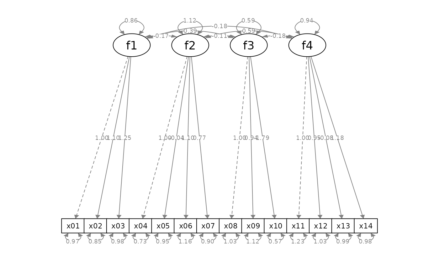 # Place standard errors on a new line
p_cfa2 <- mark_se(p_cfa, fit_cfa, sep = "\n")
plot(p_cfa2)
# Place standard errors on a new line
p_cfa2 <- mark_se(p_cfa, fit_cfa, sep = "\n")
plot(p_cfa2)
 mod_sem <-
'f1 =~ x01 + x02 + x03
f2 =~ x04 + x05 + x06 + x07
f3 =~ x08 + x09 + x10
f4 =~ x11 + x12 + x13 + x14
f3 ~ f1 + f2
f4 ~ f1 + f3
'
fit_sem <- lavaan::sem(mod_sem, sem_example)
lavaan::parameterEstimates(fit_sem)[ , c("lhs", "op", "rhs",
"est", "pvalue", "se")]
#> lhs op rhs est pvalue se
#> 1 f1 =~ x01 1.000 NA 0.000
#> 2 f1 =~ x02 1.124 0.000 0.166
#> 3 f1 =~ x03 1.310 0.000 0.191
#> 4 f2 =~ x04 1.000 NA 0.000
#> 5 f2 =~ x05 0.079 0.205 0.062
#> 6 f2 =~ x06 1.120 0.000 0.121
#> 7 f2 =~ x07 0.736 0.000 0.093
#> 8 f3 =~ x08 1.000 NA 0.000
#> 9 f3 =~ x09 0.819 0.000 0.084
#> 10 f3 =~ x10 1.230 0.000 0.112
#> 11 f4 =~ x11 1.000 NA 0.000
#> 12 f4 =~ x12 0.773 0.000 0.068
#> 13 f4 =~ x13 0.064 0.160 0.046
#> 14 f4 =~ x14 0.928 0.000 0.073
#> 15 f3 ~ f1 0.612 0.000 0.131
#> 16 f3 ~ f2 0.584 0.000 0.093
#> 17 f4 ~ f1 -0.542 0.001 0.170
#> 18 f4 ~ f3 0.980 0.000 0.127
#> 19 x01 ~~ x01 1.055 0.000 0.138
#> 20 x02 ~~ x02 1.015 0.000 0.149
#> 21 x03 ~~ x03 1.028 0.000 0.178
#> 22 x04 ~~ x04 0.933 0.000 0.144
#> 23 x05 ~~ x05 0.795 0.000 0.080
#> 24 x06 ~~ x06 0.771 0.000 0.156
#> 25 x07 ~~ x07 1.071 0.000 0.126
#> 26 x08 ~~ x08 0.976 0.000 0.134
#> 27 x09 ~~ x09 0.937 0.000 0.115
#> 28 x10 ~~ x10 1.164 0.000 0.177
#> 29 x11 ~~ x11 1.008 0.000 0.161
#> 30 x12 ~~ x12 1.033 0.000 0.131
#> 31 x13 ~~ x13 0.846 0.000 0.085
#> 32 x14 ~~ x14 0.807 0.000 0.135
#> 33 f1 ~~ f1 0.714 0.000 0.168
#> 34 f2 ~~ f2 1.277 0.000 0.229
#> 35 f3 ~~ f3 0.759 0.000 0.151
#> 36 f4 ~~ f4 1.188 0.000 0.221
#> 37 f1 ~~ f2 0.016 0.856 0.088
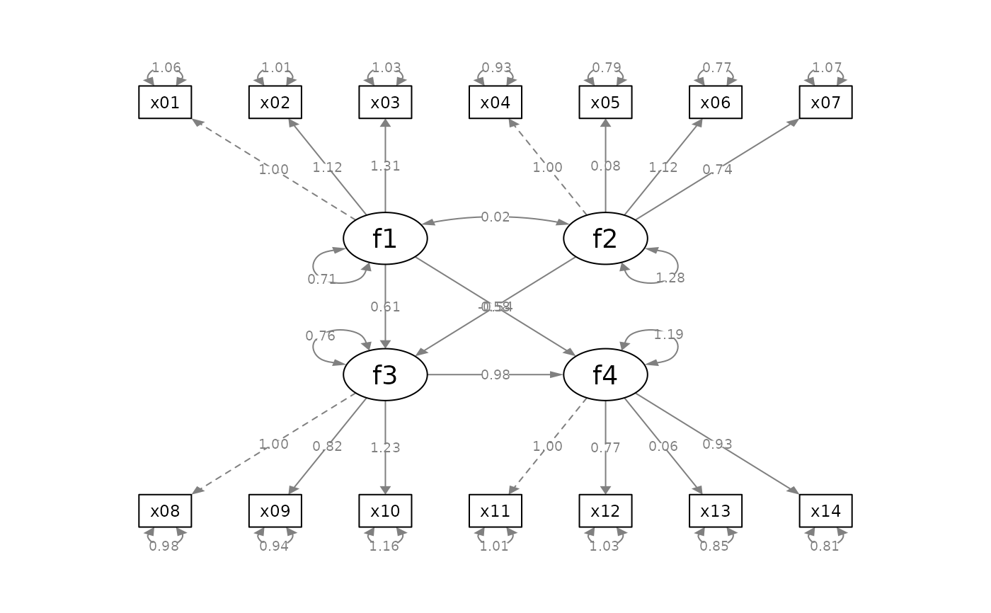
p_sem <- semPlot::semPaths(fit_sem, whatLabels = "est",
style = "ram",
nCharNodes = 0, nCharEdges = 0)
mod_sem <-
'f1 =~ x01 + x02 + x03
f2 =~ x04 + x05 + x06 + x07
f3 =~ x08 + x09 + x10
f4 =~ x11 + x12 + x13 + x14
f3 ~ f1 + f2
f4 ~ f1 + f3
'
fit_sem <- lavaan::sem(mod_sem, sem_example)
lavaan::parameterEstimates(fit_sem)[ , c("lhs", "op", "rhs",
"est", "pvalue", "se")]
#> lhs op rhs est pvalue se
#> 1 f1 =~ x01 1.000 NA 0.000
#> 2 f1 =~ x02 1.124 0.000 0.166
#> 3 f1 =~ x03 1.310 0.000 0.191
#> 4 f2 =~ x04 1.000 NA 0.000
#> 5 f2 =~ x05 0.079 0.205 0.062
#> 6 f2 =~ x06 1.120 0.000 0.121
#> 7 f2 =~ x07 0.736 0.000 0.093
#> 8 f3 =~ x08 1.000 NA 0.000
#> 9 f3 =~ x09 0.819 0.000 0.084
#> 10 f3 =~ x10 1.230 0.000 0.112
#> 11 f4 =~ x11 1.000 NA 0.000
#> 12 f4 =~ x12 0.773 0.000 0.068
#> 13 f4 =~ x13 0.064 0.160 0.046
#> 14 f4 =~ x14 0.928 0.000 0.073
#> 15 f3 ~ f1 0.612 0.000 0.131
#> 16 f3 ~ f2 0.584 0.000 0.093
#> 17 f4 ~ f1 -0.542 0.001 0.170
#> 18 f4 ~ f3 0.980 0.000 0.127
#> 19 x01 ~~ x01 1.055 0.000 0.138
#> 20 x02 ~~ x02 1.015 0.000 0.149
#> 21 x03 ~~ x03 1.028 0.000 0.178
#> 22 x04 ~~ x04 0.933 0.000 0.144
#> 23 x05 ~~ x05 0.795 0.000 0.080
#> 24 x06 ~~ x06 0.771 0.000 0.156
#> 25 x07 ~~ x07 1.071 0.000 0.126
#> 26 x08 ~~ x08 0.976 0.000 0.134
#> 27 x09 ~~ x09 0.937 0.000 0.115
#> 28 x10 ~~ x10 1.164 0.000 0.177
#> 29 x11 ~~ x11 1.008 0.000 0.161
#> 30 x12 ~~ x12 1.033 0.000 0.131
#> 31 x13 ~~ x13 0.846 0.000 0.085
#> 32 x14 ~~ x14 0.807 0.000 0.135
#> 33 f1 ~~ f1 0.714 0.000 0.168
#> 34 f2 ~~ f2 1.277 0.000 0.229
#> 35 f3 ~~ f3 0.759 0.000 0.151
#> 36 f4 ~~ f4 1.188 0.000 0.221
#> 37 f1 ~~ f2 0.016 0.856 0.088
p_sem <- semPlot::semPaths(fit_sem, whatLabels = "est",
style = "ram",
nCharNodes = 0, nCharEdges = 0)
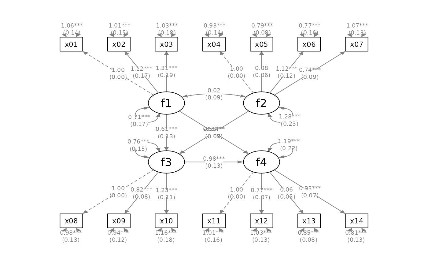
 # Mark significance, and then add standard errors
p_sem2 <- mark_sig(p_sem, fit_sem)
p_sem3 <- mark_se(p_sem2, fit_sem, sep = "\n")
plot(p_sem3)
# Mark significance, and then add standard errors
p_sem2 <- mark_sig(p_sem, fit_sem)
p_sem3 <- mark_se(p_sem2, fit_sem, sep = "\n")
plot(p_sem3)
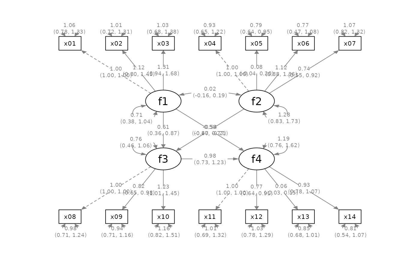
 # Add confidence intervals
p_sem4 <- mark_ci(p_sem, fit_sem, sep = "\n")
plot(p_sem4)
# Add confidence intervals
p_sem4 <- mark_ci(p_sem, fit_sem, sep = "\n")
plot(p_sem4)