Index Plot of an Arbitrary Statistic

A generic index plot function for plotting values of a column # in a matrix.

Usage

index_plot(
  object,
  column = NULL,
  plot_title = "Index Plot",
  x_label = NULL,
  cutoff_x_low = NULL,
  cutoff_x_high = NULL,
  largest_x = 1,
  absolute = FALSE,
  point_aes = list(),
  vline_aes = list(),
  hline_aes = list(),
  cutoff_line_aes = list(),
  case_label_aes = list()
)

Arguments

object: A matrix-like object, such as the output from influence_stat(), est_change(), est_change_raw(), and their counterparts for the approximate approach.
column: String. The column name of the values to be plotted.
plot_title: The title of the plot. Default is "Index Plot".
x_label: The Label for the vertical axis, for the value of column. Default is NULL. If NULL, then the label is changed to "Statistic" if absolute is FALSE, and "Absolute(Statistics)" if absolute is TRUE.
cutoff_x_low: Cases with values smaller than this value will be labeled. A cutoff line will be drawn at this value. Default is NULL. If NULL, no cutoff line will be drawn for this value.
cutoff_x_high: Cases with values larger than this value will be labeled. A cutoff line will be drawn at this value. Default is NULL. If NULL, no cutoff line will be drawn for this value.
largest_x: The number of cases with the largest absolute value on `column`` to be labelled. Default is 1. If not an integer, it will be rounded to the nearest integer.
absolute: Whether absolute values will be plotted. Useful when cases are to be compared on magnitude, ignoring sign. Default is FALSE.
point_aes: A named list of arguments to be passed to ggplot2::geom_point() to modify how to draw the points. Default is list() and internal default settings will be used.
vline_aes: A named list of arguments to be passed to ggplot2::geom_segment() to modify how to draw the line for each case in the index plot. Default is list() and internal default settings will be used.
hline_aes: A named list of arguments to be passed to ggplot2::geom_hline() to modify how to draw the horizontal line for zero case influence. Default is list() and internal default settings will be used.
cutoff_line_aes: A named list of arguments to be passed to ggplot2::geom_hline() to modify how to draw the line for user cutoff values. Default is list() and internal default settings will be used.
case_label_aes: A named list of arguments to be passed to ggrepel::geom_label_repel() to modify how to draw the labels for cases marked (based on arguments such as cutoff_x_low or largest_x). Default is list() and internal default settings will be used.

Value

A ggplot2 plot. Plotted by default. If assigned to a variable or called inside a function, it will not be plotted. Use plot() to plot it.

Details

This index plot function is for plotting any measure of influence or extremeness in a matrix. It can be used for measures not supported with other functions.

Like functions such as gcd_plot() and est_change_plot(), it supports labelling cases based on the values on the selected measure (originaL values or absolute values).

Users can also plot cases based on the absolute values. This is useful when cases are to be compared on magnitude, ignoring the sign.

Author

Shu Fai Cheung https://orcid.org/0000-0002-9871-9448.

Examples

library(lavaan)
dat <- pa_dat
# The model
mod <-
"
m1 ~ a1 * iv1 + a2 * iv2
dv ~ b * m1
a1b := a1 * b
a2b := a2 * b
"
# Fit the model
fit <- lavaan::sem(mod, dat)
summary(fit)
#> lavaan 0.6.17 ended normally after 1 iteration
#> 
#>   Estimator                                         ML
#>   Optimization method                           NLMINB
#>   Number of model parameters                         5
#> 
#>   Number of observations                           100
#> 
#> Model Test User Model:
#>                                                       
#>   Test statistic                                 6.711
#>   Degrees of freedom                                 2
#>   P-value (Chi-square)                           0.035
#> 
#> Parameter Estimates:
#> 
#>   Standard errors                             Standard
#>   Information                                 Expected
#>   Information saturated (h1) model          Structured
#> 
#> Regressions:
#>                    Estimate  Std.Err  z-value  P(>|z|)
#>   m1 ~                                                
#>     iv1       (a1)    0.215    0.106    2.036    0.042
#>     iv2       (a2)    0.522    0.099    5.253    0.000
#>   dv ~                                                
#>     m1         (b)    0.517    0.106    4.895    0.000
#> 
#> Variances:
#>                    Estimate  Std.Err  z-value  P(>|z|)
#>    .m1                0.903    0.128    7.071    0.000
#>    .dv                1.321    0.187    7.071    0.000
#> 
#> Defined Parameters:
#>                    Estimate  Std.Err  z-value  P(>|z|)
#>     a1b               0.111    0.059    1.880    0.060
#>     a2b               0.270    0.075    3.581    0.000
#> 

# --- Leave-One-Out Approach

# Fit the model n times. Each time with one case removed.
# For illustration, do this only for selected cases.
fit_rerun <- lavaan_rerun(fit, parallel = FALSE,
                          to_rerun = 1:10)
#> The expected CPU time is 0.37 second(s).
#> Could be faster if run in parallel.
# Get all default influence stats
out <- influence_stat(fit_rerun)

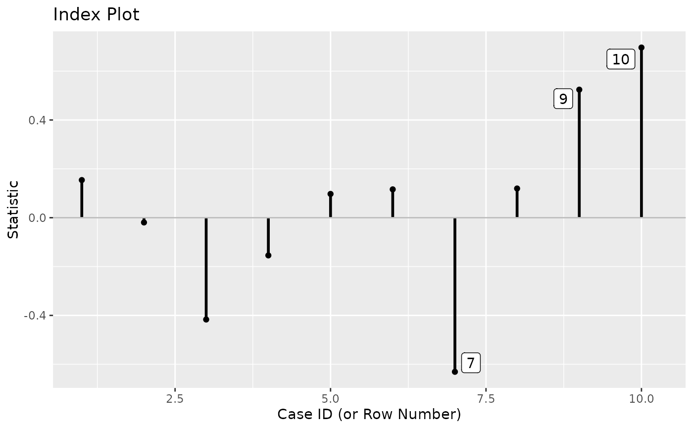
# Plot case influence on chi-square. Label the 3 cases with the influence.
index_plot(out, "chisq", largest_x = 3)


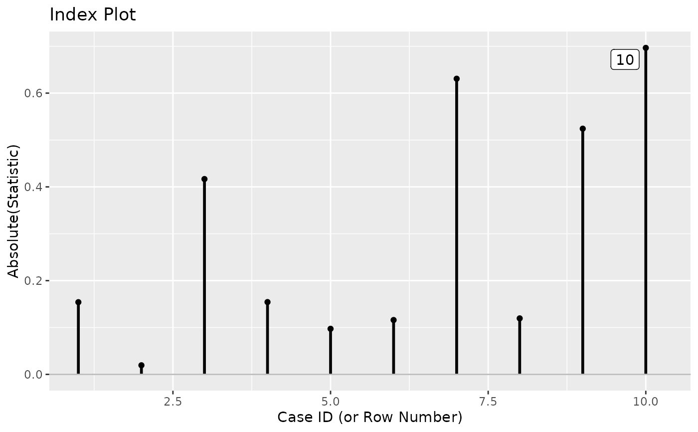
# Plot absolute case influence on chi-square.
index_plot(out, "chisq", absolute = TRUE)