Sensitivity Analysis: Arbitrary User Function

Goal

This article illustrates how to identify cases that are influential on an arbitrary statistics computed by any function, using the semfindr package .

Readers are assumed to have a basic understanding on how to use lavaan_rerun(), as illustrated in this article.

Case Influence on Any Statistic

The function user_change_raw() can be use to compute case influence measure for any statistics as long as it is provided a function that:

accepts a lavaan object (e.g., the output of lavaan::cfa() or lavaan::sem()).
returns a numeric vector of the statistics. If named, the names will be used. If not, names will be created automatically.

Different scenarios will be illustrated below.

Case 1: Reliability

We first illustrate computing case influence on reliability.

The sample dataset HolzingerSwineford1939 from the lavaan package will be used for illustration.

library(semfindr)
library(lavaan)
head(HolzingerSwineford1939)
#>   id sex ageyr agemo  school grade       x1   x2    x3       x4   x5        x6
#> 1  1   1    13     1 Pasteur     7 3.333333 7.75 0.375 2.333333 5.75 1.2857143
#> 2  2   2    13     7 Pasteur     7 5.333333 5.25 2.125 1.666667 3.00 1.2857143
#> 3  3   2    13     1 Pasteur     7 4.500000 5.25 1.875 1.000000 1.75 0.4285714
#> 4  4   1    13     2 Pasteur     7 5.333333 7.75 3.000 2.666667 4.50 2.4285714
#> 5  5   2    12     2 Pasteur     7 4.833333 4.75 0.875 2.666667 4.00 2.5714286
#> 6  6   2    14     1 Pasteur     7 5.333333 5.00 2.250 1.000000 3.00 0.8571429
#>         x7   x8       x9
#> 1 3.391304 5.75 6.361111
#> 2 3.782609 6.25 7.916667
#> 3 3.260870 3.90 4.416667
#> 4 3.000000 5.30 4.861111
#> 5 3.695652 6.30 5.916667
#> 6 4.347826 6.65 7.500000

For illustration, we add an influential case:

dat <- HolzingerSwineford1939
dat[1, c("x1", "x2", "x3")] <- dat[1, c("x1", "x2", "x3")] +
                               c(-3, +3, 0)

A confirmatory factor analysis model is to be fitted to the items x1 to x9:

mod <-
"
visual =~ x1 + x2 + x3
textual =~ x4 + x5 + x6
speed =~ x7 + x8 + x9
"
fit <- cfa(model = mod,
           data = dat)

Leave-One-Out (LOO) Results

We first do LOO analysis, fitting the model n times, n being the number of cases, each time with one case removed:

fit_rerun <- lavaan_rerun(fit)
#> The expected CPU time is 9.03 second(s).
#> Could be faster if run in parallel.

Reliability

Suppose we are interested in the reliability of the three factors. They can be computed by compRelSEM() from semTools:

library(semTools)
fit_rel <- compRelSEM(fit)
fit_rel
#>  visual textual   speed 
#>   0.594   0.885   0.688

We can compute the influence of each case using user_change_raw():

influence_rel <- user_change_raw(fit_rerun,
                                 user_function = compRelSEM)

The first argument is the output of lavaan_rerun().

The argument user_function is the argument used to compute the statistics.

No other arguments are needed in this case because compRelSEM() expects the lavaan object as the first argument.

The output is an est_change object:

influence_rel
#> 
#> -- Case Influence on User Function --
#> 
#>     id visual  id textual  id  speed
#> 1    1 -0.021 262  -0.003 140  0.011
#> 2   71  0.009 113  -0.002 194  0.010
#> 3  268 -0.008 267   0.002 209  0.008
#> 4  105  0.008   1  -0.002 240  0.008
#> 5  143  0.008  53   0.002  78 -0.007
#> 6  223  0.008 194   0.002 152  0.007
#> 7   47  0.008 254  -0.002 205  0.007
#> 8  163  0.007 217   0.002 192 -0.007
#> 9  107 -0.007 252   0.002  69 -0.006
#> 10  67 -0.007 105  -0.002  34 -0.006
#> 
#> Note:
#> - Changes are raw changes if a case is included.
#> - Only the first 10 case(s) is/are displayed. Set 'first' to NULL to display all cases.
#> - Cases sorted by the absolute changes for each variable.

The influence is computed by:

(User statistic with all case) - (User statistic without this case).

Therefore, if the value is positive for a case, the statistic, reliability in this case, is larger if this case is included.

Conversely, if the value is negative for a case, the statistic is decreases if this case is included.

The function index_plot() can be used to visualize the influence. For example, this is the plot of case influence on the reliability of visual.

Case Influence on Reliability

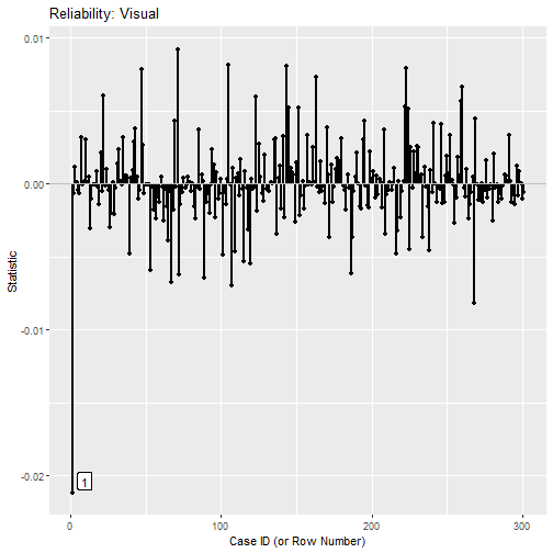
The output is a ggplot object, column needs to be set to the name of the statistic to be plotted. Refer to the help page of index_plot() for other arguments available.

As shown by both the printout and the plot, including the first case reduces the reliability of visual by 0.021.

We can verify this by fitting the model and compute the reliability without the first case:

fit_no_1 <- cfa(model = mod,
                data = dat[-1, ])
fit_rel_no_1 <- compRelSEM(fit_no_1)
# Without the first case
fit_rel_no_1
#>  visual textual   speed 
#>   0.615   0.887   0.685
# Including the first case
fit_rel
#>  visual textual   speed 
#>   0.594   0.885   0.688

Case 2: R-Squares

Suppose we use the compute case influence on R-squares. This is the sample dataset, sem_dat, comes with semfindr:

head(sem_dat)
#>           x1          x2         x3         x5         x4          x6
#> 1 -3.2135320 -0.09911249 -0.4745297 -2.8185015 -2.3237313 -0.12266637
#> 2 -0.1088671 -0.03470386 -2.2979899 -0.8178882 -0.9265397 -0.01402581
#> 3 -1.7961567 -1.58736219 -1.9552732  0.9009897 -0.5253893 -0.08915439
#> 4 -0.2033852 -2.13104958 -1.7085362 -0.7472562 -3.9749580  0.19330125
#> 5  2.2112260  1.47880579  0.2114521  0.5049098  0.2629869  2.29991139
#> 6 -1.2585361 -1.16345650 -2.9582246  0.8640491 -1.0727813 -2.07746666
#>            x7         x8         x9
#> 1  0.01778275  1.3242028  0.3511373
#> 2  1.81705005 -0.3905953 -0.5412106
#> 3  1.40417325 -0.3905477 -1.6177656
#> 4 -0.45070746 -2.3402317 -0.3714296
#> 5 -0.73314813 -0.1867083  0.4762137
#> 6  0.02449975 -0.2139832 -3.4676929
mod <-
"
f1 =~  x1 + x2 + x3
f2 =~  x4 + x5 + x6
f3 =~  x7 + x8 + x9
f2 ~ f1
f3 ~ f2 + f1
"
fit <- sem(mod,
           data = sem_dat)

The R-squares can be retrieved in different ways. For example, it can be extracted by lavInspect() from lavaan:

lavInspect(fit, what = "rsquare")
#>    x1    x2    x3    x4    x5    x6    x7    x8    x9    f2    f3 
#> 0.330 0.166 0.324 0.675 0.425 0.187 0.102 0.315 0.486 0.463 0.596

Let’s do LOO first:

fit_rerun <- lavaan_rerun(fit)
#> The expected CPU time is 10 second(s).
#> Could be faster if run in parallel.

We then call user_change_raw() to compute case influence:

influence_rsq <- user_change_raw(fit_rerun,
                                 user_function = lavInspect,
                                 what = "rsquare")

This example illustrates an advanced scenario. The function lavInspect() requires one more argument, what, to know that we want the R-squares. Such arguments require by user_function can be passed directly to user_change_raw(), which will pass them to user_function.

This is the output:

influence_rsq
#> 
#> -- Case Influence on User Function --
#> 
#>     id     x1  id     x2  id     x3  id     x4  id     x5  id     x6  id     x7
#> 1   88 -0.029 100 -0.018 112 -0.028  46 -0.045  46  0.031  61  0.016  46  0.019
#> 2   61 -0.022 125  0.017 147 -0.028  61  0.028   6 -0.022  46  0.015  27 -0.012
#> 3  120 -0.019 109 -0.014  91 -0.021  99 -0.027 178  0.019  25  0.014 110  0.012
#> 4  110  0.019  96 -0.014  61  0.020  24 -0.026 137  0.019 128 -0.014  18  0.011
#> 5   21 -0.018 149  0.013  84 -0.020 178 -0.023 110  0.018 108 -0.014  30 -0.011
#> 6  180 -0.018  75 -0.012 126 -0.017  25  0.022  25 -0.018 149 -0.013 179  0.009
#> 7  162 -0.016 116 -0.011 110  0.016  87 -0.020 200 -0.017 175 -0.013  14 -0.009
#> 8  187 -0.014 179 -0.011  46  0.015 110 -0.018 149 -0.015 164  0.012  25  0.009
#> 9   46  0.013   4  0.010  13  0.015 197 -0.018 176 -0.015  60 -0.012   3 -0.009
#> 10  59  0.012  63  0.010   6  0.014   6  0.017  70 -0.014 178  0.011  19 -0.009
#>     id     x8  id     x9  id     f2  id     f3
#> 1  106 -0.027  54 -0.030  55 -0.029 137 -0.044
#> 2  125  0.023 162 -0.027 162 -0.029  55 -0.042
#> 3   59 -0.017 134 -0.026  46  0.028   1 -0.030
#> 4   75 -0.017  66 -0.024  35 -0.027  16 -0.029
#> 5  172 -0.017  97 -0.023 149 -0.026 134 -0.027
#> 6   17  0.015  14 -0.022 119 -0.025  54  0.026
#> 7   63  0.015  46  0.022 178  0.022   6  0.024
#> 8  179  0.014 136 -0.021   3 -0.022 188 -0.024
#> 9   61  0.013  63  0.021  49 -0.021  61  0.022
#> 10  25  0.013  25 -0.018 137  0.021 121 -0.022
#> 
#> Note:
#> - Changes are raw changes if a case is included.
#> - Only the first 10 case(s) is/are displayed. Set 'first' to NULL to display all cases.
#> - Cases sorted by the absolute changes for each variable.

We can use index_plot() again. Let’s plot case influence on the R-square of f3:

Case Influence on R-Square: f3

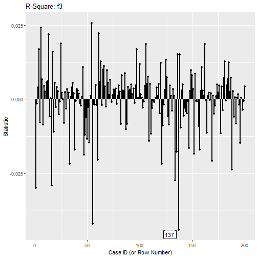
The 137th case, if included, decreases the R-square of f3 by about 0.044, as shown in both the printout and the index plot.

Final Remarks

The function user_change_raw() can also be used for function for which the lavaan-class object is not the first argument. Please refer to the help page of user_change_raw() on how to set this argument.

2025-01-25