Gets an influence_stat() output and plots selected
statistics.
Usage
gcd_plot(
  influence_out,
  cutoff_gcd = NULL,
  largest_gcd = 1,
  point_aes = list(),
  vline_aes = list(),
  cutoff_line_aes = list(),
  case_label_aes = list()
)

md_plot(
  influence_out,
  cutoff_md = FALSE,
  cutoff_md_qchisq = 0.975,
  largest_md = 1,
  point_aes = list(),
  vline_aes = list(),
  cutoff_line_aes = list(),
  case_label_aes = list()
)

gcd_gof_plot(
  influence_out,
  fit_measure,
  cutoff_gcd = NULL,
  cutoff_fit_measure = NULL,
  largest_gcd = 1,
  largest_fit_measure = 1,
  point_aes = list(),
  hline_aes = list(),
  cutoff_line_gcd_aes = list(),
  cutoff_line_fit_measures_aes = list(),
  case_label_aes = list()
)

gcd_gof_md_plot(
  influence_out,
  fit_measure,
  cutoff_md = FALSE,
  cutoff_fit_measure = NULL,
  circle_size = 2,
  cutoff_md_qchisq = 0.975,
  cutoff_gcd = NULL,
  largest_gcd = 1,
  largest_md = 1,
  largest_fit_measure = 1,
  point_aes = list(),
  hline_aes = list(),
  cutoff_line_md_aes = list(),
  cutoff_line_gcd_aes = list(),
  cutoff_line_fit_measures_aes = list(),
  case_label_aes = list()
)
Arguments
- influence_out
The output from
influence_stat().- cutoff_gcd
Cases with generalized Cook's distance or approximate generalized Cook's distance larger than this value will be labeled. Default is
NULL. IfNULL, no cutoff line will be drawn.- largest_gcd
The number of cases with the largest generalized Cook's distance or approximate generalized Cook's distance to be labelled. Default is 1. If not an integer, it will be rounded to the nearest integer.
- point_aes
A named list of arguments to be passed to
ggplot2::geom_point()to modify how to draw the points. Default islist()and internal default settings will be used.- vline_aes
A named list of arguments to be passed to
ggplot2::geom_segment()to modify how to draw the line for each case in the index plot. Default islist()and internal default settings will be used.- cutoff_line_aes
A named list of arguments to be passed to
ggplot2::geom_vline()orggplot2::geom_hline()to modify how to draw the line for user cutoff value. Default islist()and internal default settings will be used.- case_label_aes
A named list of arguments to be passed to
ggrepel::geom_label_repel()to modify how to draw the labels for cases marked (based on arguments such ascutoff_gcdorlargest_gcd). Default islist()and internal default settings will be used.- cutoff_md
Cases with Mahalanobis distance larger than this value will be labeled. If it is
TRUE, the (cutoff_md_qchisqx 100)th percentile of the chi-square distribution with the degrees of freedom equal to the number of variables will be used. Default isFALSE, no cutoff value.- cutoff_md_qchisq
This value multiplied by 100 is the percentile to be used for labeling case based on Mahalanobis distance. Default is .975.
- largest_md
The number of cases with the largest Mahalanobis distance to be labelled. Default is 1. If not an integer, it will be rounded to the nearest integer.
- fit_measure
The fit measure to be used in a plot. Use the name in the
lavaan::fitMeasures()function. No default value.- cutoff_fit_measure
Cases with
fit_measurelarger than this cutoff in magnitude will be labeled. No default value and must be specified.- largest_fit_measure
The number of cases with the largest selected fit measure change in magnitude to be labelled. Default is
If not an integer, it will be rounded to the nearest integer.
- hline_aes
A named list of arguments to be passed to
ggplot2::geom_hline()to modify how to draw the horizontal line for zero case influence. Default islist()and internal default settings will be used.- cutoff_line_gcd_aes
Similar to
cutoff_line_aesbut control the line for the cutoff value of gCD.- cutoff_line_fit_measures_aes
Similar to
cutoff_line_aesbut control the line for the cutoff value of the selected fit measure.- circle_size
The size of the largest circle when the size of a circle is controlled by a statistic.
- cutoff_line_md_aes
Similar to
cutoff_line_aesbut control the line for the cutoff value of the Mahalanobis distance.
Value
A ggplot2 plot. Plotted by default. If assigned to a variable
or called inside a function, it will not be plotted. Use plot() to
plot it.
Details
The output of influence_stat() is simply a matrix.
Therefore, these functions will work for any matrix provided. Row
number will be used on the x-axis if applicable. However, case
identification values in the output from influence_stat() will
be used for labeling individual cases.
The default settings for the plots
should be good enough for diagnostic
purpose. If so desired, users can
use the *_aes arguments to nearly
fully customize all the major
elements of the plots, as they would
do for building a ggplot2 plot.
Functions
gcd_plot(): Index plot of generalized Cook's distance.md_plot(): Index plot of Mahalanobis distance.gcd_gof_plot(): Plot the case influence of the selected fit measure against generalized Cook's distance.gcd_gof_md_plot(): Bubble plot of the case influence of the selected fit measure against Mahalanobis distance, with the size of a bubble determined by generalized Cook's distance.
References
Cheung, S. F., & Lai, M. H. C. (2026). semfindr:
An R package for identifying influential cases in
structural equation modeling.
Multivariate Behavioral Research.
Advance online publication.
doi:10.1080/00273171.2026.2634293
Pek, J., & MacCallum, R. (2011). Sensitivity analysis in structural equation models: Cases and their influence. Multivariate Behavioral Research, 46(2), 202-228. doi:10.1080/00273171.2011.561068
Author
Shu Fai Cheung https://orcid.org/0000-0002-9871-9448.
Examples
library(lavaan)
dat <- pa_dat
# The model
mod <-
"
m1 ~ a1 * iv1 + a2 * iv2
dv ~ b * m1
a1b := a1 * b
a2b := a2 * b
"
# Fit the model
fit <- lavaan::sem(mod, dat)
summary(fit)
#> lavaan 0.6-21 ended normally after 1 iteration
#>
#> Estimator ML
#> Optimization method NLMINB
#> Number of model parameters 5
#>
#> Number of observations 100
#>
#> Model Test User Model:
#>
#> Test statistic 6.711
#> Degrees of freedom 2
#> P-value (Chi-square) 0.035
#>
#> Parameter Estimates:
#>
#> Standard errors Standard
#> Information Expected
#> Information saturated (h1) model Structured
#>
#> Regressions:
#> Estimate Std.Err z-value P(>|z|)
#> m1 ~
#> iv1 (a1) 0.215 0.106 2.036 0.042
#> iv2 (a2) 0.522 0.099 5.253 0.000
#> dv ~
#> m1 (b) 0.517 0.106 4.895 0.000
#>
#> Variances:
#> Estimate Std.Err z-value P(>|z|)
#> .m1 0.903 0.128 7.071 0.000
#> .dv 1.321 0.187 7.071 0.000
#>
#> Defined Parameters:
#> Estimate Std.Err z-value P(>|z|)
#> a1b 0.111 0.059 1.880 0.060
#> a2b 0.270 0.075 3.581 0.000
#>
# Fit the model n times. Each time with one case removed.
# For illustration, do this only for selected cases.
fit_rerun <- lavaan_rerun(fit, parallel = FALSE,
to_rerun = 1:10)
#> The expected CPU time is 0.45 second(s).
#> Could be faster if run in parallel.
# Get all default influence stats
out <- influence_stat(fit_rerun)
head(out)
#> chisq cfi rmsea tli a1
#> 1 0.15407944 -0.0019968390 0.0017700811 -0.0049920976 0.024466586
#> 2 -0.01944571 0.0011486763 -0.0010912308 0.0028716908 0.007153846
#> 3 -0.41673808 0.0082048797 -0.0074508538 0.0205121991 -0.038282397
#> 4 -0.15430823 0.0036670450 -0.0032789585 0.0091676124 -0.024048244
#> 5 0.09730667 0.0002954311 0.0008280336 0.0007385778 0.066686613
#> 6 0.11601736 -0.0010911517 0.0011378622 -0.0027278793 0.004007056
#> a2 b m1~~m1 dv~~dv gcd md
#> 1 -0.0300705396 0.051965997 -0.03663071 0.01717427 0.005891665 1.9107778
#> 2 0.0034230301 -0.013043400 -0.06744802 -0.05802199 0.008147128 0.4442464
#> 3 -0.0401051535 -0.029790144 -0.06335355 -0.04479763 0.009834826 3.7867385
#> 4 -0.0031358865 0.021674577 -0.05137193 -0.04379632 0.005610493 1.0653437
#> 5 0.0278462201 0.032782898 0.04979077 -0.06598323 0.013001467 1.9803351
#> 6 0.0009699846 0.009509592 -0.06910195 -0.05422999 0.007823146 0.2875484
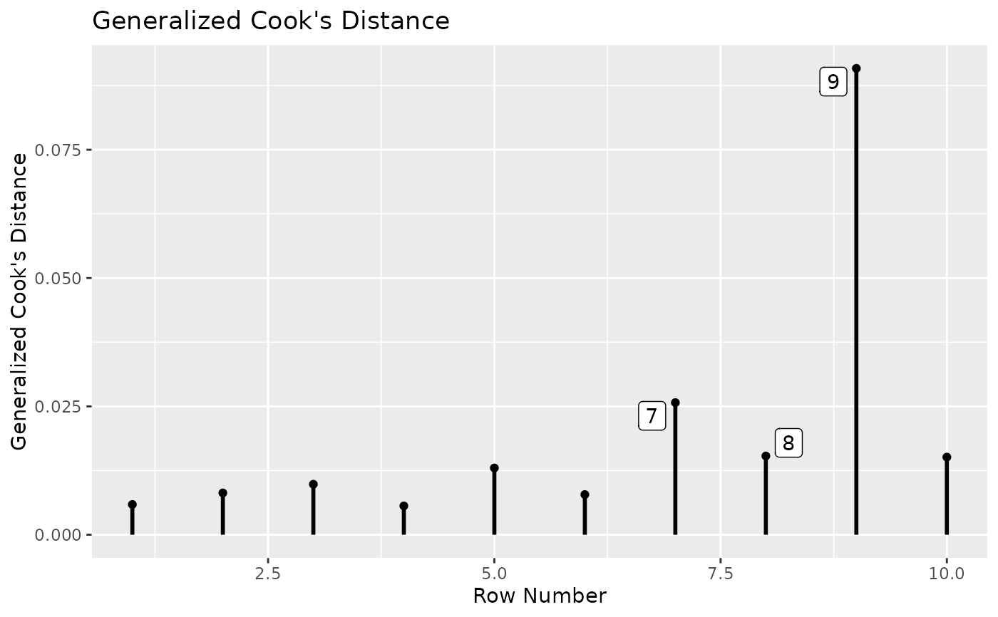
# Plot generalized Cook's distance. Label the 3 cases with the largest distances.
gcd_plot(out, largest_gcd = 3)
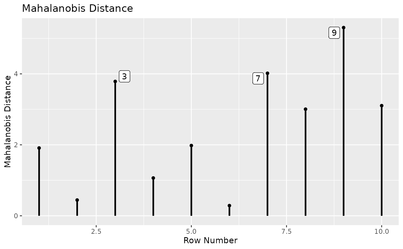
 # Plot Mahalanobis distance. Label the 3 cases with the largest distances.
md_plot(out, largest_md = 3)
# Plot Mahalanobis distance. Label the 3 cases with the largest distances.
md_plot(out, largest_md = 3)
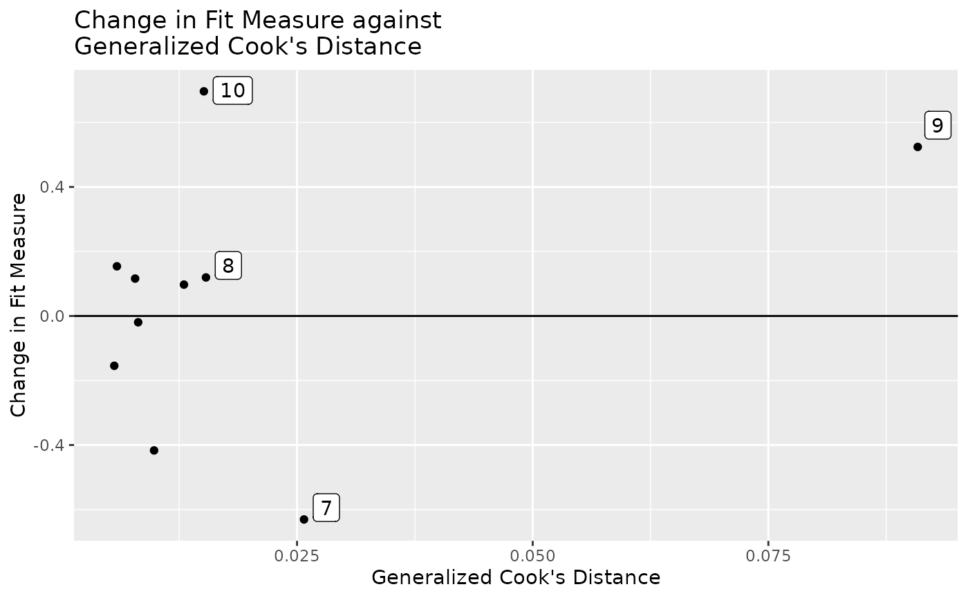
 # Plot case influence on model chi-square against generalized Cook's distance.
# Label the 3 cases with the largest absolute influence.
# Label the 3 cases with the largest generalized Cook's distance.
gcd_gof_plot(out, fit_measure = "chisq", largest_gcd = 3,
largest_fit_measure = 3)
# Plot case influence on model chi-square against generalized Cook's distance.
# Label the 3 cases with the largest absolute influence.
# Label the 3 cases with the largest generalized Cook's distance.
gcd_gof_plot(out, fit_measure = "chisq", largest_gcd = 3,
largest_fit_measure = 3)
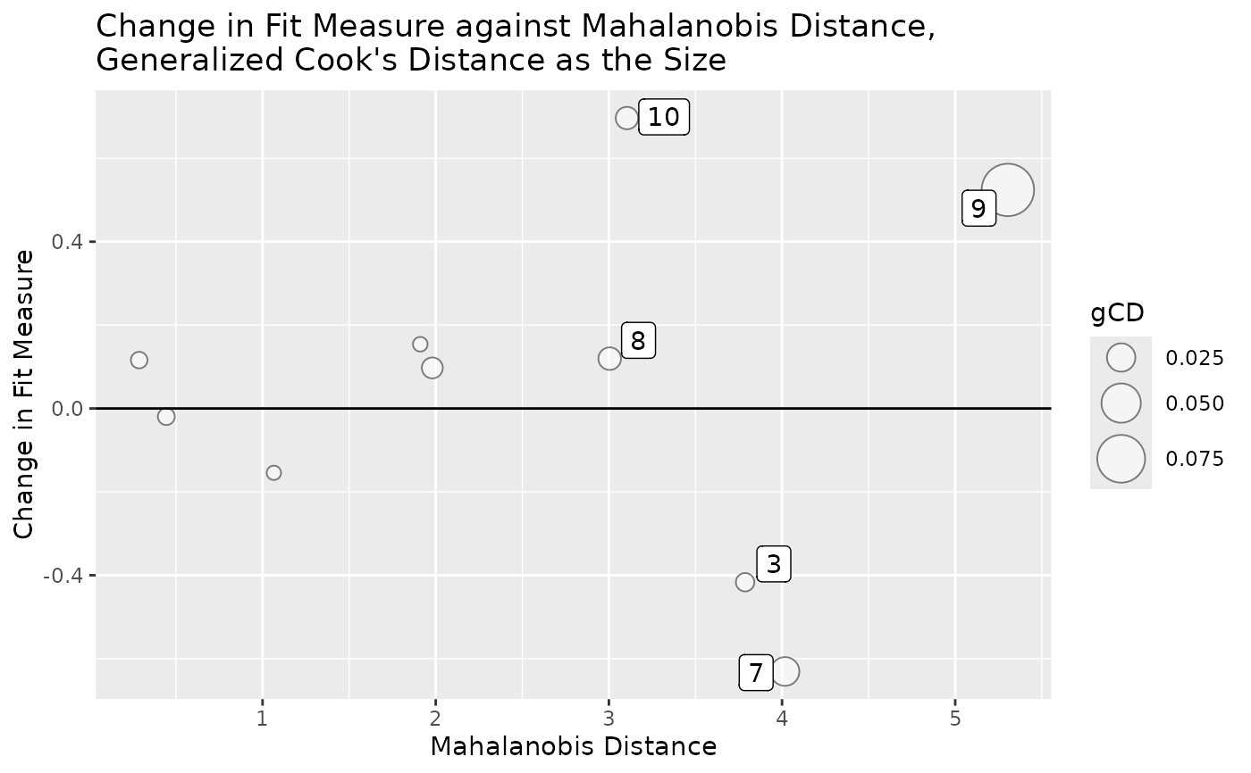
 # Plot case influence on model chi-square against Mahalanobis distance.
# Size of bubble determined by generalized Cook's distance.
# Label the 3 cases with the largest absolute influence.
# Label the 3 cases with the largest Mahalanobis distance.
# Label the 3 cases with the largest generalized Cook's distance.
gcd_gof_md_plot(out, fit_measure = "chisq",
largest_gcd = 3,
largest_fit_measure = 3,
largest_md = 3,
circle_size = 10)
# Plot case influence on model chi-square against Mahalanobis distance.
# Size of bubble determined by generalized Cook's distance.
# Label the 3 cases with the largest absolute influence.
# Label the 3 cases with the largest Mahalanobis distance.
# Label the 3 cases with the largest generalized Cook's distance.
gcd_gof_md_plot(out, fit_measure = "chisq",
largest_gcd = 3,
largest_fit_measure = 3,
largest_md = 3,
circle_size = 10)
 # Use the approximate method that does not require refitting the model.
# Fit the model
fit <- lavaan::sem(mod, dat)
summary(fit)
#> lavaan 0.6-21 ended normally after 1 iteration
#>
#> Estimator ML
#> Optimization method NLMINB
#> Number of model parameters 5
#>
#> Number of observations 100
#>
#> Model Test User Model:
#>
#> Test statistic 6.711
#> Degrees of freedom 2
#> P-value (Chi-square) 0.035
#>
#> Parameter Estimates:
#>
#> Standard errors Standard
#> Information Expected
#> Information saturated (h1) model Structured
#>
#> Regressions:
#> Estimate Std.Err z-value P(>|z|)
#> m1 ~
#> iv1 (a1) 0.215 0.106 2.036 0.042
#> iv2 (a2) 0.522 0.099 5.253 0.000
#> dv ~
#> m1 (b) 0.517 0.106 4.895 0.000
#>
#> Variances:
#> Estimate Std.Err z-value P(>|z|)
#> .m1 0.903 0.128 7.071 0.000
#> .dv 1.321 0.187 7.071 0.000
#>
#> Defined Parameters:
#> Estimate Std.Err z-value P(>|z|)
#> a1b 0.111 0.059 1.880 0.060
#> a2b 0.270 0.075 3.581 0.000
#>
out <- influence_stat(fit)
head(out)
#> chisq cfi rmsea tli m1~iv1
#> 1 0.15956516 -0.0020929857 0.0018614175 -0.005232464 0.024713396
#> 2 -0.01892880 0.0011399150 -0.0010827859 0.002849787 0.007254736
#> 3 -0.38907022 0.0077186573 -0.0070161267 0.019296643 -0.037982774
#> 4 -0.15078126 0.0036048257 -0.0032221332 0.009012064 -0.024353717
#> 5 0.09685352 0.0003104848 0.0008205378 0.000776212 0.067010210
#> 6 0.11602751 -0.0010913266 0.0011380304 -0.002728316 0.004065567
#> m1~iv2 dv~m1 m1~~m1 dv~~dv gcd_approx md
#> 1 -0.030383580 0.052370026 -0.03784100 0.01630488 0.005850455 1.9107778
#> 2 0.003469647 -0.013223396 -0.06916983 -0.05953293 0.008312026 0.4442464
#> 3 -0.039820283 -0.030150418 -0.06518369 -0.04609708 0.009904544 3.7867385
#> 4 -0.003172373 0.021948305 -0.05277394 -0.04504791 0.005719499 1.0653437
#> 5 0.027951233 0.032981527 0.04860722 -0.06774242 0.012793226 1.9803351
#> 6 0.000983731 0.009640981 -0.07086163 -0.05565453 0.007984573 0.2875484
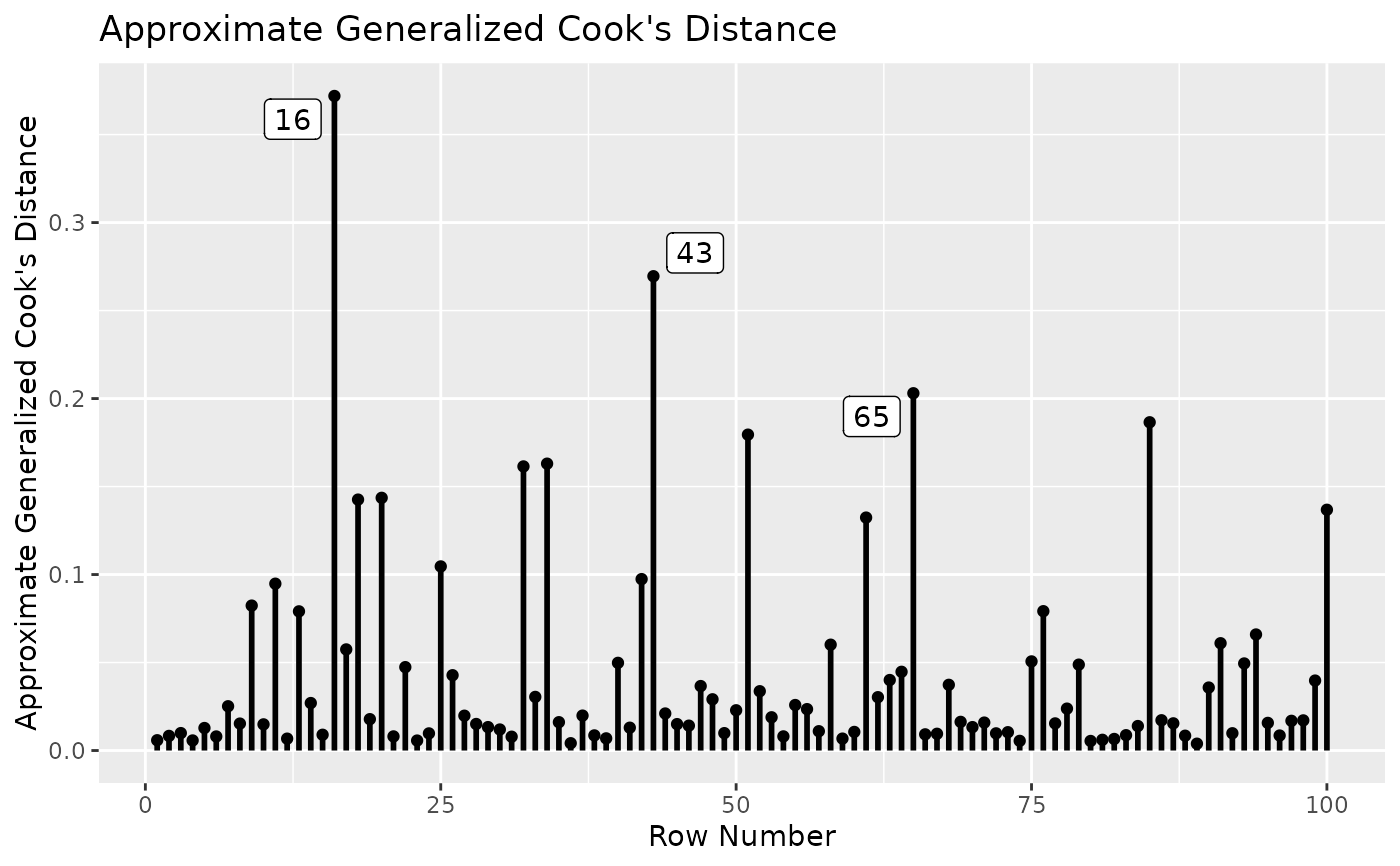
# Plot approximate generalized Cook's distance.
# Label the 3 cases with the largest values.
gcd_plot(out, largest_gcd = 3)
# Use the approximate method that does not require refitting the model.
# Fit the model
fit <- lavaan::sem(mod, dat)
summary(fit)
#> lavaan 0.6-21 ended normally after 1 iteration
#>
#> Estimator ML
#> Optimization method NLMINB
#> Number of model parameters 5
#>
#> Number of observations 100
#>
#> Model Test User Model:
#>
#> Test statistic 6.711
#> Degrees of freedom 2
#> P-value (Chi-square) 0.035
#>
#> Parameter Estimates:
#>
#> Standard errors Standard
#> Information Expected
#> Information saturated (h1) model Structured
#>
#> Regressions:
#> Estimate Std.Err z-value P(>|z|)
#> m1 ~
#> iv1 (a1) 0.215 0.106 2.036 0.042
#> iv2 (a2) 0.522 0.099 5.253 0.000
#> dv ~
#> m1 (b) 0.517 0.106 4.895 0.000
#>
#> Variances:
#> Estimate Std.Err z-value P(>|z|)
#> .m1 0.903 0.128 7.071 0.000
#> .dv 1.321 0.187 7.071 0.000
#>
#> Defined Parameters:
#> Estimate Std.Err z-value P(>|z|)
#> a1b 0.111 0.059 1.880 0.060
#> a2b 0.270 0.075 3.581 0.000
#>
out <- influence_stat(fit)
head(out)
#> chisq cfi rmsea tli m1~iv1
#> 1 0.15956516 -0.0020929857 0.0018614175 -0.005232464 0.024713396
#> 2 -0.01892880 0.0011399150 -0.0010827859 0.002849787 0.007254736
#> 3 -0.38907022 0.0077186573 -0.0070161267 0.019296643 -0.037982774
#> 4 -0.15078126 0.0036048257 -0.0032221332 0.009012064 -0.024353717
#> 5 0.09685352 0.0003104848 0.0008205378 0.000776212 0.067010210
#> 6 0.11602751 -0.0010913266 0.0011380304 -0.002728316 0.004065567
#> m1~iv2 dv~m1 m1~~m1 dv~~dv gcd_approx md
#> 1 -0.030383580 0.052370026 -0.03784100 0.01630488 0.005850455 1.9107778
#> 2 0.003469647 -0.013223396 -0.06916983 -0.05953293 0.008312026 0.4442464
#> 3 -0.039820283 -0.030150418 -0.06518369 -0.04609708 0.009904544 3.7867385
#> 4 -0.003172373 0.021948305 -0.05277394 -0.04504791 0.005719499 1.0653437
#> 5 0.027951233 0.032981527 0.04860722 -0.06774242 0.012793226 1.9803351
#> 6 0.000983731 0.009640981 -0.07086163 -0.05565453 0.007984573 0.2875484
# Plot approximate generalized Cook's distance.
# Label the 3 cases with the largest values.
gcd_plot(out, largest_gcd = 3)
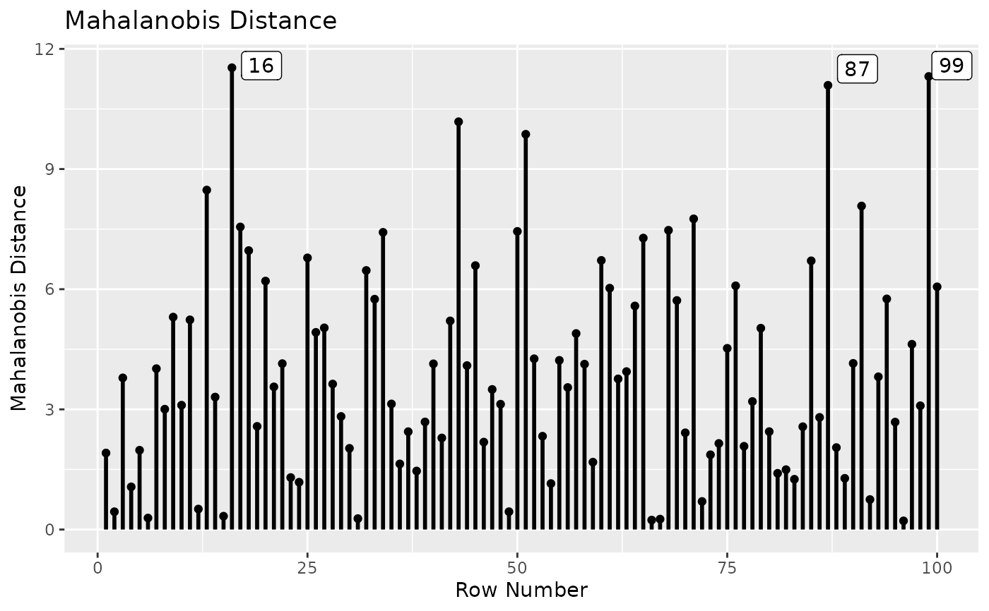
 # Plot Mahalanobis distance.
# Label the 3 cases with the largest values.
md_plot(out, largest_md = 3)
# Plot Mahalanobis distance.
# Label the 3 cases with the largest values.
md_plot(out, largest_md = 3)
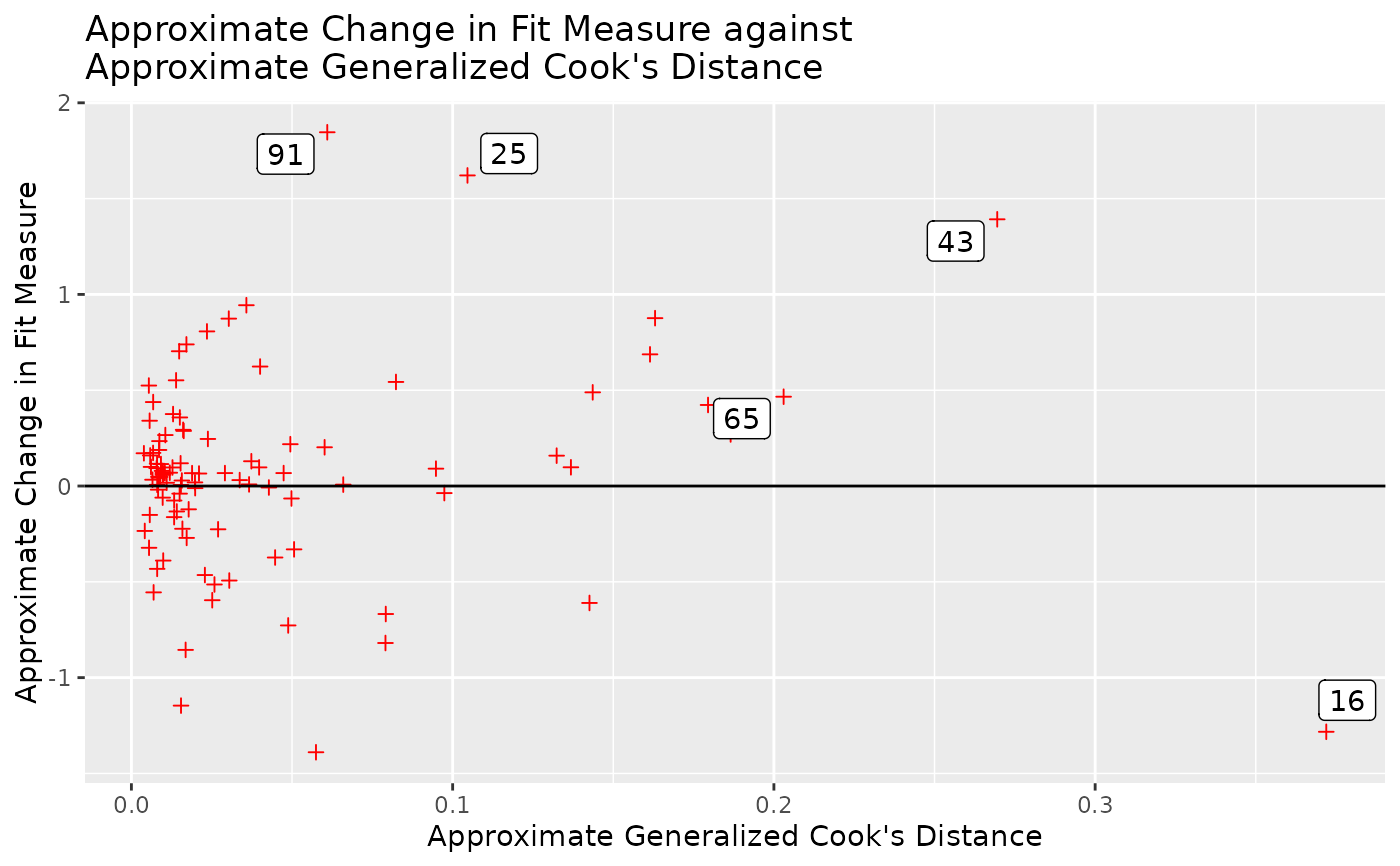
 # Plot approximate case influence on model chi-square against
# approximate generalized Cook's distance.
# Label the 3 cases with the largest absolute approximate case influence.
# Label the 3 cases with the largest approximate generalized Cook's distance.
gcd_gof_plot(out, fit_measure = "chisq", largest_gcd = 3,
largest_fit_measure = 3)
# Plot approximate case influence on model chi-square against
# approximate generalized Cook's distance.
# Label the 3 cases with the largest absolute approximate case influence.
# Label the 3 cases with the largest approximate generalized Cook's distance.
gcd_gof_plot(out, fit_measure = "chisq", largest_gcd = 3,
largest_fit_measure = 3)
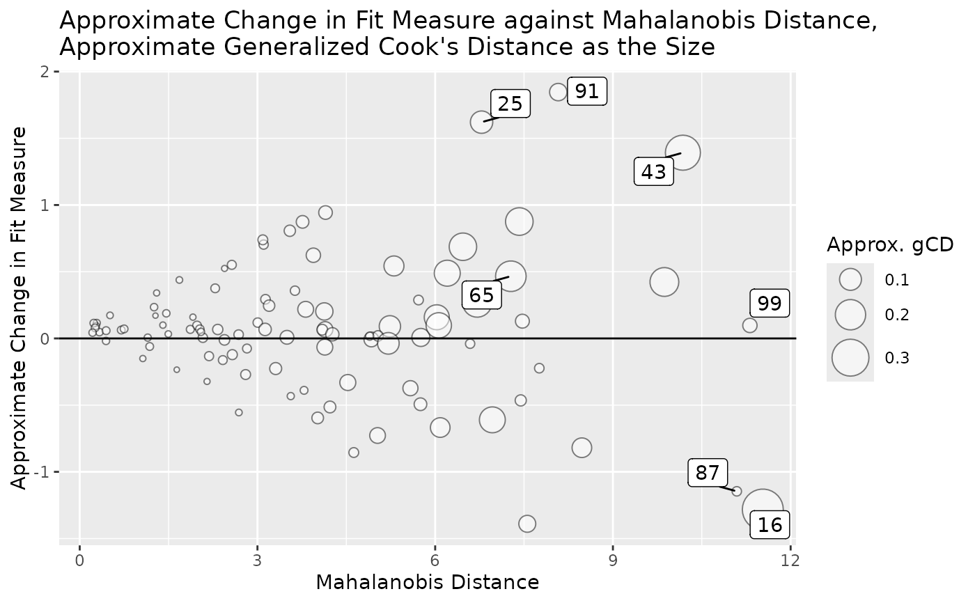
 # Plot approximate case influence on model chi-square against Mahalanobis distance.
# The size of a bubble determined by approximate generalized Cook's distance.
# Label the 3 cases with the largest absolute approximate case influence.
# Label the 3 cases with the largest Mahalanobis distance.
# Label the 3 cases with the largest approximate generalized Cook's distance.
gcd_gof_md_plot(out, fit_measure = "chisq",
largest_gcd = 3,
largest_fit_measure = 3,
largest_md = 3,
circle_size = 10)
# Plot approximate case influence on model chi-square against Mahalanobis distance.
# The size of a bubble determined by approximate generalized Cook's distance.
# Label the 3 cases with the largest absolute approximate case influence.
# Label the 3 cases with the largest Mahalanobis distance.
# Label the 3 cases with the largest approximate generalized Cook's distance.
gcd_gof_md_plot(out, fit_measure = "chisq",
largest_gcd = 3,
largest_fit_measure = 3,
largest_md = 3,
circle_size = 10)
 # Customize elements in the plot.
# For example, change the color and shape of the points.
gcd_gof_plot(out, fit_measure = "chisq", largest_gcd = 3,
largest_fit_measure = 3,
point_aes = list(shape = 3, color = "red"))
# Customize elements in the plot.
# For example, change the color and shape of the points.
gcd_gof_plot(out, fit_measure = "chisq", largest_gcd = 3,
largest_fit_measure = 3,
point_aes = list(shape = 3, color = "red"))