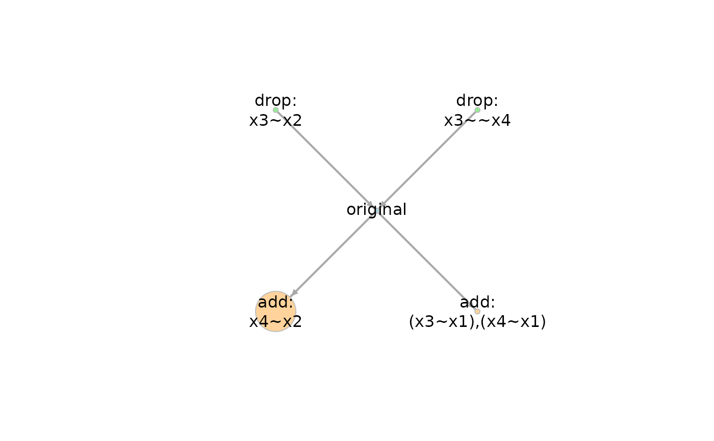
Plot a Network of Models

Plot a network of models generated by model_graph().

Usage

# S3 method for class 'model_graph'
plot(x, ...)

Arguments

x

The output of model_graph(). (Named x because it is required in the naming of arguments of the plot generic function.)

...

Additional arguments, passed to the plot-method of an igraph object.

Value

NULL. Called for its side effect.

Details

This function is the plot method of model_graph objects, the output of model_graph().

For now, it simply passes the object to plot-method of an igraph object. This function is created for possible customization of the plot in the future.

See also

model_graph()

Examples

library(lavaan)

dat <- dat_path_model

mod <-
"
x3 ~ a*x1 + b*x2
x4 ~ a*x1
ab := a*b
"

fit <- sem(mod, dat_path_model, fixed.x = TRUE)

out <- model_set(fit)
#> 
#> Generate 2 less restrictive model(s):
#> 
  |                                                  | 0 % ~calculating  
  |+++++++++++++++++++++++++                         | 50% ~00s          
  |++++++++++++++++++++++++++++++++++++++++++++++++++| 100% elapsed=00s  
#> 
#> Generate 2 more restrictive model(s):
#> 
  |                                                  | 0 % ~calculating  
  |+++++++++++++++++++++++++                         | 50% ~00s          
  |++++++++++++++++++++++++++++++++++++++++++++++++++| 100% elapsed=00s  
#> 
#> Check for duplicated models (5 model[s] to check):
#> 
  |                                                        
  |                                                  |   0%
  |                                                        
  |+++++                                             |  10%
  |                                                        
  |++++++++++                                        |  20%
  |                                                        
  |+++++++++++++++                                   |  30%
  |                                                        
  |++++++++++++++++++++                              |  40%
  |                                                        
  |+++++++++++++++++++++++++                         |  50%
  |                                                        
  |++++++++++++++++++++++++++++++                    |  60%
  |                                                        
  |+++++++++++++++++++++++++++++++++++               |  70%
  |                                                        
  |++++++++++++++++++++++++++++++++++++++++          |  80%
  |                                                        
  |+++++++++++++++++++++++++++++++++++++++++++++     |  90%
  |                                                        
  |++++++++++++++++++++++++++++++++++++++++++++++++++| 100%
#> 
#> Fit the 5 model(s) (duplicated models removed):
out
#> 
#> Call:
#> model_set(sem_out = fit)
#> 
#> Number of model(s) fitted           : 5
#> Number of model(s) converged        : 5
#> Number of model(s) passed post.check: 5
#> 
#> The models (sorted by BPP):
#>                      model_df df_diff Prior     BIC   BPP   cfi rmsea
#> add: x4~x2                  1       1 0.200 400.291 1.000 1.000 0.017
#> original                    2       0 0.200 431.452 0.000 0.736 0.417
#> add: (x3~x1),(x4~x1)        1       1 0.200 435.397 0.000 0.733 0.593
#> drop: x3~~x4                3      -1 0.200 441.229 0.000 0.634 0.401
#> drop: x3~x2                 3      -1 0.200 455.926 0.000 0.522 0.458
#> 
#> Note:
#> - BIC: Bayesian Information Criterion.
#> - BPP: BIC posterior probability.
#> - model_df: Model degrees of freedom.
#> - df_diff: Difference in df compared to the original/target model.
#> - To show cumulative BPPs, call print() with 'cumulative_bpp = TRUE'.
#> - At least one model has fixed.x = TRUE. The models are not checked for
#>   equivalence.
#> - Since Version 0.1.3.5, the default values of exclude_feedback and
#>   exclude_xy_cov changed to TRUE. Set them to FALSE to reproduce
#>   results from previous versions.

g <- model_graph(out)
plot(g)