Generate an 'igraph' object from a 'model_set' object.
Usage
model_graph(
  object,
  node_size_by_x = TRUE,
  x = NULL,
  node_size = 5,
  min_size = 5,
  max_size = 35,
  color_original = "lightblue",
  color_add = "burlywood1",
  color_drop = "lightgreen",
  color_others = "lightgrey",
  color_label = "black",
  node_label_size = 1,
  original = "original",
  drop_redundant_direct_paths = TRUE,
  label_arrow_by_df = NULL,
  arrow_label_size = 1,
  weight_arrows_by_df = c("inverse", "normal", "none"),
  arrow_min_width = 0.5,
  arrow_max_width = 2,
  progress = TRUE,
  short_names = FALSE,
  min_bpp_labelled = NULL,
  ...
)
Arguments
- object
Must be a
model_set-class object for now.- node_size_by_x
Logical. Whether node (vertex) sizes are determined by a variable. Default is
TRUE. Seexbelow on how size is determined.- x
If not
NULL, it should be a numeric vector of length equal to the number of models. The node sizes will be proportional to the values ofx, offset bymin_size. IfNULL, the default, the BIC posterior probabilities stored inobjectwill be retrieved.- node_size
If
node_size_by_xisFALSE, this is the size for all nodes.- min_size
The minimum size of a node. Default is 5.
- max_size
The maximum size of a node. Default is 35.
- color_original
The color of node of the original model. Default is
"lightblue".- color_add
The color of the nodes of models formed by adding one or more free parameters to the original model. Default is
"burlywood1".- color_drop
The color of the nodes of models formed by dropping one or more free parameters from the original model. Default is
"lightgreen".- color_others
The color of other models not specified above. Default is
"grey50".- color_label
The color of the text labels of the nodes. Default is
"black".- node_label_size
The size of the labels of the nodes. Default is 1.
- original
String. The name of the original model (target model). Default is
"original".- drop_redundant_direct_paths
Logical. Whether the redundant direct path between two models. A direct path is redundant if two models are also connected through at least one another model. Default is
TRUE.- label_arrow_by_df
If
TRUE, then an arrow (edge) is always labelled by the difference in model dfs. IfFALSE, then no arrows are labelled. IfNULL, then arrows are labelled when not all differences in model dfs are equal to one. Default isNULL.- arrow_label_size
The size of the labels of the arrows (edges), if labelled. Default is 1.
- weight_arrows_by_df
String. Use if model df differences are stored. If
"inverse", larger the difference in model df, narrower an arrow. That is, more similar two models are, thicker the arrow. If"normal", larger the difference in model df, wider an arrow. If"none", then arrow width is constant, set toarrow_max_width. Default is"inverse".- arrow_min_width
If
weight_arrows_by_dfis not"none", this is the minimum width of an arrow.- arrow_max_width
If
weight_arrows_by_dfis not"none", this is the maximum width of an arrow. Ifweight_arrows_by_dfis"none", this is the width of all arrows.- progress
Whether a progress bar will be displayed for some steps (e.g., checking for nested relations). Default is
TRUE.- short_names
If
TRUEand short model names are stored, they will be used as model labels. Please print the object withshort_names = TRUEto find the corresponding full model names.- min_bpp_labelled
If not
NULL, this is the minimum BPP for a model to be labelled. Models with BPP less than this value will not be labelled. Useful when the number of models is large.- ...
Optional arguments. Not used for now.
Value
A model_graph-class object that
can be used as as an igraph-object,
with a plot method (plot.model_graph())
with settings
suitable for plotting a network
of models with BIC posterior probabilities
computed.
Details
It extracts the model list stored
in object, creates an adjacency
matrix, and then creates an igraph
object customized for visualizing
model relations.
Construction of the Graph
This is the default way to construct
the graph when the model set is
automatically by model_set().
Each model is connected by an arrow, pointing from one model to another model that
a. can be formed by adding one or more free parameter, or
b. can be formed by releasing one or more equality constraint between two parameters.
c. has nested relation with this model as determined by the method proposed by Bentler and Satorra (2010), if the models are not generated internally.
That is, it points to a model with more degrees of freedom (more complicated), and is nested within that model in either parameter sense or covariance sense.
By default, the size of the node for each model is scaled by its BIC posterior probability, if available. See The Size of a Node below.
If a model is designated as the original (target) model, than he original model, the models with more degrees of freedom than the original model, and the models with fewer degrees of freedom than the original models, are colored differently.
The default layout is the Sugiyama layout, with simpler models (models with fewer degrees of freedom) on the top. The lower a model is in the network, the more the degrees of freedom it has. This layout is suitable for showing the nested relations of the models. Models on the same level (layer) horizontally have the same model df.
The output is an igraph object.
Users can customize it in any way
they want using functions from
the igraph package.
If a model has no nested relation with all other model, it will not be connected to other models.
If no model is named original
(default is "original"), then no
model is colored as the original model.
User-Provided Models
If object contained one or more
user-provided models which are not
generated automatically by
model_set() or similar functions
(e.g., gen_models()), then the
method by Bentler and Satorra (2010)
will be used to determine model
relations. Models connected by an
arrow has a nested relation based on
the NET method by Bentler and Satorra
(2010). An internal function inspired
by the net function from the
semTools package is used to
implement the NET method.
References
Bentler, P. M., & Satorra, A. (2010). Testing model nesting and equivalence. Psychological Methods, 15(2), 111–123. doi:10.1037/a0019625 Asparouhov, T., & Muthén, B. (2019). Nesting and Equivalence Testing for Structural Equation Models. Structural Equation Modeling: A Multidisciplinary Journal, 26(2), 302–309. doi:10.1080/10705511.2018.1513795
Author
Shu Fai Cheung https://orcid.org/0000-0002-9871-9448
The internal function for nesting
inspired by the net function
from the semTools package,
which was developed by
Terrence D. Jorgensen.
Examples
library(lavaan)
mod <-
"
m1 ~ x
y ~ m1
"
fit <- sem(mod, dat_serial_4, fixed.x = TRUE)
out <- model_set(fit)
#>
#> Generate 1 less restrictive model(s):
#>
| | 0 % ~calculating
|++++++++++++++++++++++++++++++++++++++++++++++++++| 100% elapsed=00s
#>
#> Generate 2 more restrictive model(s):
#>
| | 0 % ~calculating
|+++++++++++++++++++++++++ | 50% ~00s
|++++++++++++++++++++++++++++++++++++++++++++++++++| 100% elapsed=00s
#>
#> Check for duplicated models (4 model[s] to check):
#>
|
| | 0%
|
|++++++++ | 17%
|
|+++++++++++++++++ | 33%
|
|+++++++++++++++++++++++++ | 50%
|
|+++++++++++++++++++++++++++++++++ | 67%
|
|++++++++++++++++++++++++++++++++++++++++++ | 83%
|
|++++++++++++++++++++++++++++++++++++++++++++++++++| 100%
#>
#> Fit the 4 model(s) (duplicated models removed):
out
#>
#> Call:
#> model_set(sem_out = fit)
#>
#> Number of model(s) fitted : 4
#> Number of model(s) converged : 4
#> Number of model(s) passed post.check: 4
#>
#> The models (sorted by BPP):
#> model_df df_diff Prior BIC BPP cfi rmsea srmr
#> original 1 0 0.250 370.869 0.880 1.000 0.000 0.014
#> add: y~x 0 1 0.250 374.847 0.120 1.000 0.000 0.000
#> drop: y~m1 2 -1 0.250 431.244 0.000 0.615 0.564 0.353
#> drop: m1~x 2 -1 0.250 469.045 0.000 0.387 0.712 0.390
#>
#> Note:
#> - BIC: Bayesian Information Criterion.
#> - BPP: BIC posterior probability.
#> - model_df: Model degrees of freedom.
#> - df_diff: Difference in df compared to the original/target model.
#> - To show cumulative BPPs, call print() with 'cumulative_bpp = TRUE'.
#> - At least one model has fixed.x = TRUE. The models are not checked for
#> equivalence.
#> - Since Version 0.1.6.3, the default ways to handle factor loadings
#> have changed. Check the NEWS by news(package = 'modelbpp') to see how
#> to reproduce results from previous versions.
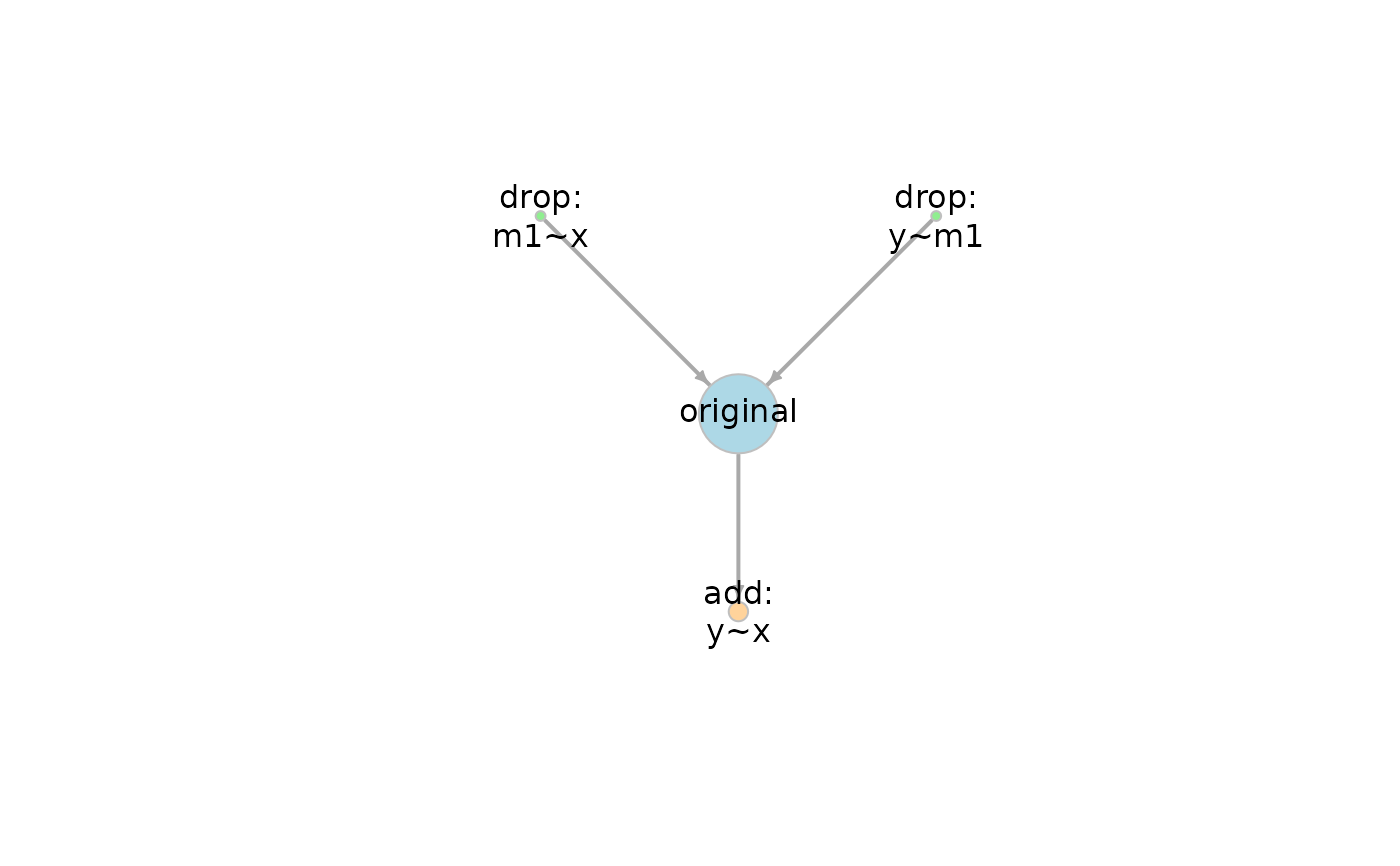
g <- model_graph(out)
plot(g)