Introduction
This article illustrates how to use model_set() and
other functions from the package modelbpp
to:
Fit a set of neighboring models, each has one more or one less degree of freedom than the original fitted model.
Compute the BIC posterior probability (BPP), for each model (Wu et al., 2020).
Use BPP to assess to what extent each model is supported by the data, compared to all other models under consideration.
An introduction to the package can be found in the following article:
- Pesigan, I. J. A., Cheung, S. F., Wu, H., Chang, F., & Leung, S. O. (2026). How plausible is my model? Assessing model plausibility of structural equation models using Bayesian posterior probabilities (BPP). Behavior Research Methods, 58(3), Article 73. https://doi.org/10.3758/s13428-025-02921-x
Workflow
Fit an SEM model, the original model, as usual in
lavaan.-
Call
model_set()on the output from Step 1. It will automatically do the following:Enumerate the neighboring models of the original model.
Fit all the models and compute their BIC posterior probabilities (BPPs).
-
Examine the results by:
printing the output of
model_set(), orgenerating a graph using
model_graph().
Example
This is a sample dataset, dat_serial_4_weak, with four
variables:
library(modelbpp)
head(dat_serial_4_weak)
#>             x         m1         m2          y
#> 1  0.09107195  1.2632493  0.7823926  0.3252093
#> 2 -1.96063838 -0.7745526  0.2002867 -0.6379673
#> 3  0.20184014  0.2238152  0.2374072  0.4205998
#> 4 -2.25521708  0.1185732 -0.1727878  0.9320889
#> 5 -0.15321350  0.1509888  1.1251386  0.6892537
#> 6 -2.00640303 -0.1595208 -0.1553136 -0.2364792
Step 1: Fit the Original Model
Fit this original model, a serial mediation model, with one direct
path, from x to y:
library(lavaan)
#> This is lavaan 0.6-21
#> lavaan is FREE software! Please report any bugs.
mod1 <-
"
m1 ~ x
m2 ~ m1
y ~ m2 + x
"
fit1 <- sem(mod1, dat_serial_4_weak)
This the summary:
summary(fit1,
        fit.measures = TRUE)
#> lavaan 0.6-21 ended normally after 1 iteration
#>
#>   Estimator                                         ML
#>   Optimization method                           NLMINB
#>   Number of model parameters                         7
#>
#>   Number of observations                           100
#>
#> Model Test User Model:
#>
#>   Test statistic                                 3.376
#>   Degrees of freedom                                 2
#>   P-value (Chi-square)                           0.185
#>
#> Model Test Baseline Model:
#>
#>   Test statistic                                39.011
#>   Degrees of freedom                                 6
#>   P-value                                        0.000
#>
#> User Model versus Baseline Model:
#>
#>   Comparative Fit Index (CFI)                    0.958
#>   Tucker-Lewis Index (TLI)                       0.875
#>
#> Loglikelihood and Information Criteria:
#>
#>   Loglikelihood user model (H0)               -216.042
#>   Loglikelihood unrestricted model (H1)       -214.354
#>
#>   Akaike (AIC)                                 446.084
#>   Bayesian (BIC)                               464.320
#>   Sample-size adjusted Bayesian (SABIC)        442.212
#>
#> Root Mean Square Error of Approximation:
#>
#>   RMSEA                                          0.083
#>   90 Percent confidence interval - lower         0.000
#>   90 Percent confidence interval - upper         0.232
#>   P-value H_0: RMSEA <= 0.050                    0.261
#>   P-value H_0: RMSEA >= 0.080                    0.628
#>
#> Standardized Root Mean Square Residual:
#>
#>   SRMR                                           0.050
#>
#> Parameter Estimates:
#>
#>   Standard errors                             Standard
#>   Information                                 Expected
#>   Information saturated (h1) model          Structured
#>
#> Regressions:
#>                    Estimate  Std.Err  z-value  P(>|z|)
#>   m1 ~
#>     x                 0.187    0.059    3.189    0.001
#>   m2 ~
#>     m1                0.231    0.091    2.537    0.011
#>   y ~
#>     m2                0.341    0.089    3.835    0.000
#>     x                 0.113    0.052    2.188    0.029
#>
#> Variances:
#>                    Estimate  Std.Err  z-value  P(>|z|)
#>    .m1                0.278    0.039    7.071    0.000
#>    .m2                0.254    0.036    7.071    0.000
#>    .y                 0.213    0.030    7.071    0.000
The fit is acceptable, though the RMSEA is marginal (CFI = 0.958, RMSEA = 0.083).
Step 2: Call model_set()
Use model_set() to find the neighboring models differ
from the target model by one on model degrees of freedom, fit them, and
compute the BPPs:
out1 <- model_set(fit1)Step 3: Examine the Results
To examine the results, just print the output:
out1
#>
#> Call:
#> model_set(sem_out = fit1)
#>
#> Number of model(s) fitted           : 7
#> Number of model(s) converged        : 7
#> Number of model(s) passed post.check: 7
#>
#> The models (sorted by BPP):
#>             model_df df_diff Prior     BIC   BPP   cfi rmsea  srmr
#> original           2       0 0.143 464.320 0.323 0.958 0.083 0.050
#> drop: y~x          3      -1 0.143 464.340 0.320 0.848 0.129 0.095
#> add: y~m1          1       1 0.143 465.900 0.147 1.000 0.000 0.018
#> drop: m2~m1        3      -1 0.143 465.953 0.143 0.800 0.148 0.116
#> add: m2~x          1       1 0.143 468.575 0.038 0.939 0.142 0.046
#> drop: m1~x         3      -1 0.143 469.403 0.025 0.695 0.183 0.124
#> drop: y~m2         3      -1 0.143 473.291 0.004 0.577 0.216 0.133
#>
#> Note:
#> - BIC: Bayesian Information Criterion.
#> - BPP: BIC posterior probability.
#> - model_df: Model degrees of freedom.
#> - df_diff: Difference in df compared to the original/target model.
#> - To show cumulative BPPs, call print() with 'cumulative_bpp = TRUE'.
#> - At least one model has fixed.x = TRUE. The models are not checked for
#>   equivalence.
#> - Since Version 0.1.6.3, the default ways to handle factor loadings
#>   have changed. Check the NEWS by news(package = 'modelbpp') to see how
#>   to reproduce results from previous versions.
The total number of models examined, including the original model, is 7.
(Note: The total number of models was 9 in previous version. Please refer to the Note in the printout for the changes.)
The BIC posterior probabilities (BPPs) suggest that the original
model is indeed the most probable model based on BPP. However, the model
with the direct path dropped, drop: y~x, only has slightly
lower BPP (0.320)
This suggests that, with equal prior probabilities (Wu et al., 2020), the support for the model with the direct and without the direct path have similar support from the data based on BPP.
Alternatively, we can use model_graph() to visualize the
BPPs and model relations graphically:
graph1 <- model_graph(out1)
plot(graph1)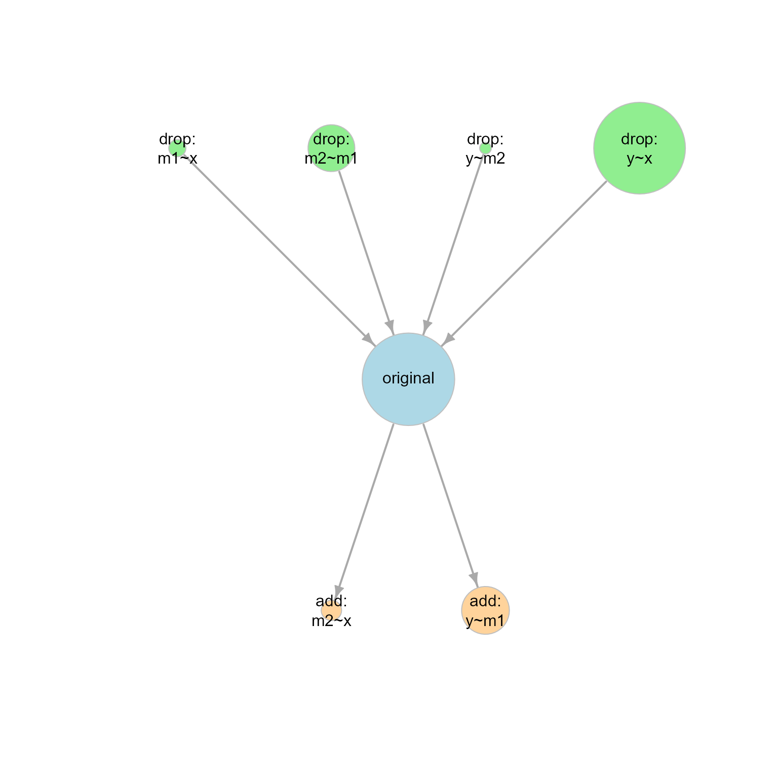
plot of chunk graph1
Each node (circle) represents one model. The larger the BPP, the larger the node.
The arrow points from a simpler model (a model with larger model df) to a more complicated model (a model with smaller model df). If two models are connected by an arrow, then one model can be formed from another model by adding or removing one free parameter (e.g., adding or removing one path).
Repeat Step 2 with User Prior
In real studies, not all models are equally probable before having data (i.e., not all models have equal prior probabilities). A researcher fits the original model because
its prior probability is higher than other models, at least other neighboring models (otherwise, it is not worthy of collecting data assess thi original model), but
the prior probability is not so high to eliminate the need for collecting data to see how much it is supported by data.
Suppose we decide that the prior probability of the original model is .50: probable, but still needs data to decide whether it is empirically supported
This can be done by setting prior_sem_out to the desired
prior probability when calling model_set():
out1_prior <- model_set(fit1,
                        prior_sem_out = .50)
The prior probabilities of all other models are equal. Therefore, with nine models and the prior of the target model being .50, the prior probability of the other eight model is (1 - .50) / 8 or .0625.
This is the printout:
out1_prior
#>
#> Call:
#> model_set(sem_out = fit1, prior_sem_out = 0.5)
#>
#> Number of model(s) fitted           : 7
#> Number of model(s) converged        : 7
#> Number of model(s) passed post.check: 7
#>
#> The models (sorted by BPP):
#>             model_df df_diff Prior     BIC   BPP   cfi rmsea  srmr
#> original           2       0 0.500 464.320 0.741 0.958 0.083 0.050
#> drop: y~x          3      -1 0.083 464.340 0.122 0.848 0.129 0.095
#> add: y~m1          1       1 0.083 465.900 0.056 1.000 0.000 0.018
#> drop: m2~m1        3      -1 0.083 465.953 0.055 0.800 0.148 0.116
#> add: m2~x          1       1 0.083 468.575 0.015 0.939 0.142 0.046
#> drop: m1~x         3      -1 0.083 469.403 0.010 0.695 0.183 0.124
#> drop: y~m2         3      -1 0.083 473.291 0.001 0.577 0.216 0.133
#>
#> Note:
#> - BIC: Bayesian Information Criterion.
#> - BPP: BIC posterior probability.
#> - model_df: Model degrees of freedom.
#> - df_diff: Difference in df compared to the original/target model.
#> - To show cumulative BPPs, call print() with 'cumulative_bpp = TRUE'.
#> - At least one model has fixed.x = TRUE. The models are not checked for
#>   equivalence.
#> - Since Version 0.1.6.3, the default ways to handle factor loadings
#>   have changed. Check the NEWS by news(package = 'modelbpp') to see how
#>   to reproduce results from previous versions.
If the prior of the target is set to .50, then, taking into account both the prior probabilities and the data, the target model is strongly supported by the data.
This is the output of model_graph():
graph1_prior <- model_graph(out1_prior)
plot(graph1_prior)
plot of chunk out1_prior
Advanced Options
More Neighboring Models
If desired, we can enumerate models “farther away” from the target model. For example, we can set the maximum difference in model df to 2, to include models having two more or two less df than the original model:
out1_df2 <- model_set(fit1,
                      df_change_add = 2,
                      df_change_drop = 2)
This is the printout. By default, when there are more than 20 models, only the top 20 models on BPP will be printed:
out1_df2
#>
#> Call:
#> model_set(sem_out = fit1, df_change_add = 2, df_change_drop = 2)
#>
#> Number of model(s) fitted           : 14
#> Number of model(s) converged        : 14
#> Number of model(s) passed post.check: 14
#>
#> The models (sorted by BPP):
#>                  model_df df_diff Prior     BIC   BPP   cfi rmsea  srmr
#> original                2       0 0.071 464.320 0.269 0.958 0.083 0.050
#> drop: y~x               3      -1 0.071 464.340 0.267 0.848 0.129 0.095
#> add: y~m1               1       1 0.071 465.900 0.122 1.000 0.000 0.018
#> drop: m2~m1             3      -1 0.071 465.953 0.119 0.800 0.148 0.116
#> drop: m2~m1;y~x         4      -2 0.071 465.973 0.118 0.690 0.160 0.149
#> add: m2~x               1       1 0.071 468.575 0.032 0.939 0.142 0.046
#> drop: m1~x              3      -1 0.071 469.403 0.021 0.695 0.183 0.124
#> drop: m1~x;y~x          4      -2 0.071 469.423 0.021 0.585 0.185 0.144
#> add: m2~x;y~m1          0       2 0.071 470.154 0.015 1.000 0.000 0.000
#> drop: m1~x;m2~m1        4      -2 0.071 471.036 0.009 0.536 0.196 0.160
#> drop: y~m2              3      -1 0.071 473.291 0.003 0.577 0.216 0.133
#> drop: y~m2;y~x          4      -2 0.071 474.819 0.001 0.422 0.218 0.170
#> drop: m2~m1;y~m2        4      -2 0.071 474.924 0.001 0.419 0.219 0.163
#> drop: m1~x;y~m2         4      -2 0.071 478.374 0.000 0.314 0.238 0.183
#>
#> Note:
#> - BIC: Bayesian Information Criterion.
#> - BPP: BIC posterior probability.
#> - model_df: Model degrees of freedom.
#> - df_diff: Difference in df compared to the original/target model.
#> - To show cumulative BPPs, call print() with 'cumulative_bpp = TRUE'.
#> - At least one model has fixed.x = TRUE. The models are not checked for
#>   equivalence.
#> - Since Version 0.1.6.3, the default ways to handle factor loadings
#>   have changed. Check the NEWS by news(package = 'modelbpp') to see how
#>   to reproduce results from previous versions.
The number of models examined, including the original model, is 14.
This is the output of model_graph():
graph1_df2 <- model_graph(out1_df2,
                          node_label_size = .75)
plot(graph1_df2)
plot of chunk graph1_df2
Note: Due to the number of nodes, node_label_size is
used to reduce the size of the labels.
Excluding Some Parameters From the Search
When calling model_set(), users can specify parameters
that must be excluded from the list to be added
(must_not_add), or must not be dropped
(must_not_drop).
For example, suppose it is well established that m1~x
exists and should not be dropped, we can exclude it when calling
model_set()
out1_no_m1_x <- model_set(fit1,
                          must_not_drop = "m1~x")
This is the output:
out1_no_m1_x
#>
#> Call:
#> model_set(sem_out = fit1, must_not_drop = "m1~x")
#>
#> Number of model(s) fitted           : 6
#> Number of model(s) converged        : 6
#> Number of model(s) passed post.check: 6
#>
#> The models (sorted by BPP):
#>             model_df df_diff Prior     BIC   BPP   cfi rmsea  srmr
#> original           2       0 0.167 464.320 0.331 0.958 0.083 0.050
#> drop: y~x          3      -1 0.167 464.340 0.328 0.848 0.129 0.095
#> add: y~m1          1       1 0.167 465.900 0.150 1.000 0.000 0.018
#> drop: m2~m1        3      -1 0.167 465.953 0.147 0.800 0.148 0.116
#> add: m2~x          1       1 0.167 468.575 0.040 0.939 0.142 0.046
#> drop: y~m2         3      -1 0.167 473.291 0.004 0.577 0.216 0.133
#>
#> Note:
#> - BIC: Bayesian Information Criterion.
#> - BPP: BIC posterior probability.
#> - model_df: Model degrees of freedom.
#> - df_diff: Difference in df compared to the original/target model.
#> - To show cumulative BPPs, call print() with 'cumulative_bpp = TRUE'.
#> - At least one model has fixed.x = TRUE. The models are not checked for
#>   equivalence.
#> - Since Version 0.1.6.3, the default ways to handle factor loadings
#>   have changed. Check the NEWS by news(package = 'modelbpp') to see how
#>   to reproduce results from previous versions.
The number of models reduced to 14.
This is the plot:
out1_no_m1_x <- model_graph(out1_no_m1_x)
plot(out1_no_m1_x)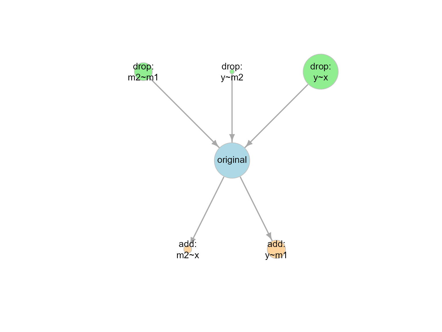
plot of chunk out1_no_m1_x
Models With Constraints
If the original model has equality constraints, they will be included in the search for neighboring models, by default. That is, removing one equality constraint between two models is considered as a model with an increase of 1 df.
Recompute BPPs Without Refitting the Models
Users can examine the impact of the prior probability of the original
model without refitting the models, by using the output of
model_set() as the input, using the
model_set_out argument:
out1_new_prior <- model_set(model_set_out = out1,
                            prior_sem_out = .50)
The results are identical to calling model_set() with
the original lavaan output as the input:
out1_new_prior
#>
#> Call:
#> model_set(model_set_out = out1, prior_sem_out = 0.5)
#>
#> Number of model(s) fitted           : 7
#> Number of model(s) converged        : 7
#> Number of model(s) passed post.check: 7
#>
#> The models (sorted by BPP):
#>             model_df df_diff Prior     BIC   BPP   cfi rmsea  srmr
#> original           2       0 0.500 464.320 0.741 0.958 0.083 0.050
#> drop: y~x          3      -1 0.083 464.340 0.122 0.848 0.129 0.095
#> add: y~m1          1       1 0.083 465.900 0.056 1.000 0.000 0.018
#> drop: m2~m1        3      -1 0.083 465.953 0.055 0.800 0.148 0.116
#> add: m2~x          1       1 0.083 468.575 0.015 0.939 0.142 0.046
#> drop: m1~x         3      -1 0.083 469.403 0.010 0.695 0.183 0.124
#> drop: y~m2         3      -1 0.083 473.291 0.001 0.577 0.216 0.133
#>
#> Note:
#> - BIC: Bayesian Information Criterion.
#> - BPP: BIC posterior probability.
#> - model_df: Model degrees of freedom.
#> - df_diff: Difference in df compared to the original/target model.
#> - To show cumulative BPPs, call print() with 'cumulative_bpp = TRUE'.
#> - At least one model has fixed.x = TRUE. The models are not checked for
#>   equivalence.
#> - Since Version 0.1.6.3, the default ways to handle factor loadings
#>   have changed. Check the NEWS by news(package = 'modelbpp') to see how
#>   to reproduce results from previous versions.
Many Neighboring Models
When a model has a lot of free parameters, the number of neighboring
models can be large and it will take a long time to fit all of them.
Users can enable parallel processing by setting parallel to
TRUE when calling model_set().
More Options
Please refer to the help page of model_set() for options
available.