Diagnostic Plots of Bootstrap Estimates

Introduction

This document introduces the function plot_boot(), and related helpers, from the package semhelpinghands. They are used for generating plots of distribution of bootstrap estimates, as suggested by Rousselet et al. (2021), to check if there is anything unusual in the bootstrap distribution, such as bootstrap estimates that are unusually extreme compared to other estimates.

Data and Model

A mediation model example modified from the official lavaan website is used (https://lavaan.ugent.be/tutorial/mediation.html).

library(lavaan)
#> This is lavaan 0.6-17
#> lavaan is FREE software! Please report any bugs.
set.seed(12345)
n <- 100
X <- rnorm(n)
M <- .30 * X + sqrt(1 - .30^2) * rnorm(n)
Y <- .60 * M + sqrt(1 - .60^2) * rnorm(n)
Data <- data.frame(X = X,
                   Y = Y,
                   M = M)
model <-
"
# direct effect
  Y ~ c*X
# mediator
  M ~ a*X
  Y ~ b*M
# indirect effect (a*b)
  ab := a*b
# total effect
  total := c + (a*b)
"

This model is fitted with se = "bootstrap" and 5000 replication. (Change ncpus to a value appropriate for the system running it.)

fit <- sem(model,
           data = Data,
           se = "bootstrap",
           bootstrap = 5000,
           parallel = "snow",
           ncpus = 4,
           iseed = 1234)

(Note that having a warning for some bootstrap runs is normal. The failed runs will not be used in forming the confidence intervals.)

This is the bootstrap confidence intervals:

parameterEstimates(fit)
#>     lhs op     rhs label   est    se     z pvalue ci.lower ci.upper
#> 1     Y  ~       X     c 0.008 0.071 0.117  0.906   -0.135    0.141
#> 2     M  ~       X     a 0.390 0.076 5.133  0.000    0.235    0.534
#> 3     Y  ~       M     b 0.505 0.087 5.814  0.000    0.331    0.668
#> 4     Y ~~       Y       0.541 0.076 7.121  0.000    0.383    0.682
#> 5     M ~~       M       0.911 0.117 7.798  0.000    0.674    1.135
#> 6     X ~~       X       1.230 0.000    NA     NA    1.230    1.230
#> 7    ab :=     a*b    ab 0.197 0.049 3.986  0.000    0.106    0.296
#> 8 total := c+(a*b) total 0.205 0.081 2.519  0.012    0.040    0.361

Plot Bootstrap Distribution

Free Parameters

To plot the distribution of bootstrap estimates of free a parameter (not user-defined parameter, i.e., not ab), call plot_boot(). The following is a sample call to plot the bootstrap estimates of the b path:

library(semhelpinghands)
plot_boot(fit,
          param = "b",
          standardized = FALSE,
          qq_dot_size = 1)

These are the required arguments:

The first argument is the output of lavaan.
The argument param should be the name of the parameter to be plotted, as appeared in a call to coef().
The argument standardized is required. It indicates whether the bootstrap estimates from the standardized solution are to be plotted.

The argument qq_dot_size is optional, for controlling the size of the points in the normal QQ-plot.

This is the plot

#> 
#> Attaching package: 'semhelpinghands'
#> The following object is masked from 'package:base':
#> 
#>     sort_by

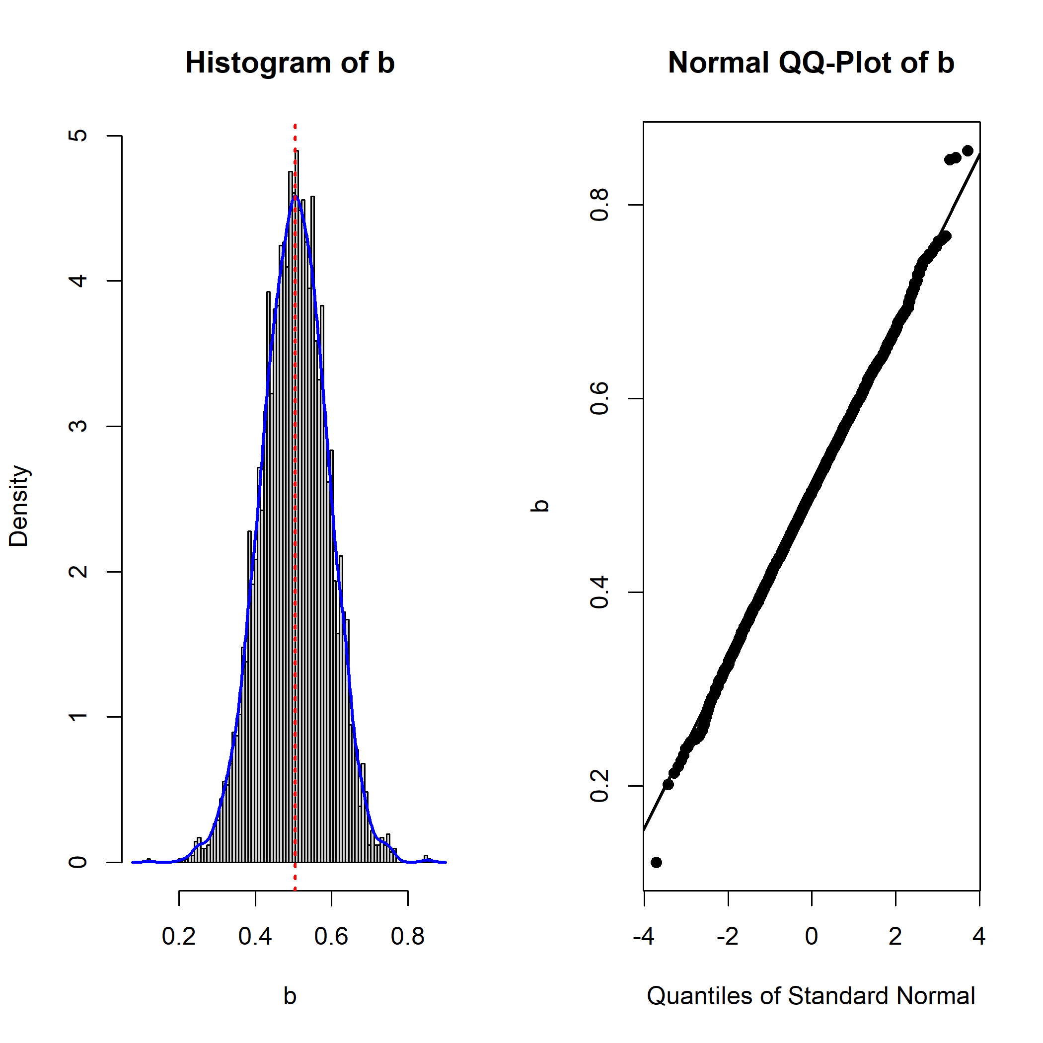
The plot is similar to that of the output of boot::boot(). The left panel is a histogram with:

A red dotted line to represent the point estimate of the parameter (the estimate of b in the lavaan output in this example).
A kernel density plot (blue line) of the distribution.

The right panel is a normal QQ-plot generated by qqnorm() and qqline(). If the distribution is normal, the points should lie on the line. Deviation from a normal distribution will be manifested as points deviate from the line vertically, usually at the lower or upper end of the distribution.

User-Defined Parameters

Only the bootstrap estimates of free parameters are stored by lavaan. To plot the distribution of bootstrap estimates, call store_boot_def() first to compute the bootstrap estimates of user-defined parameters and store them back to the output of lavaan.¹

fit <- store_boot_def(fit)

Once computed and stored, plot_boot() can be used again. For example, to plot the distribution of ab, the indirect effect, just set param to "ab".

plot_boot(fit,
          param = "ab",
          standardized = FALSE,
          qq_dot_size = 1)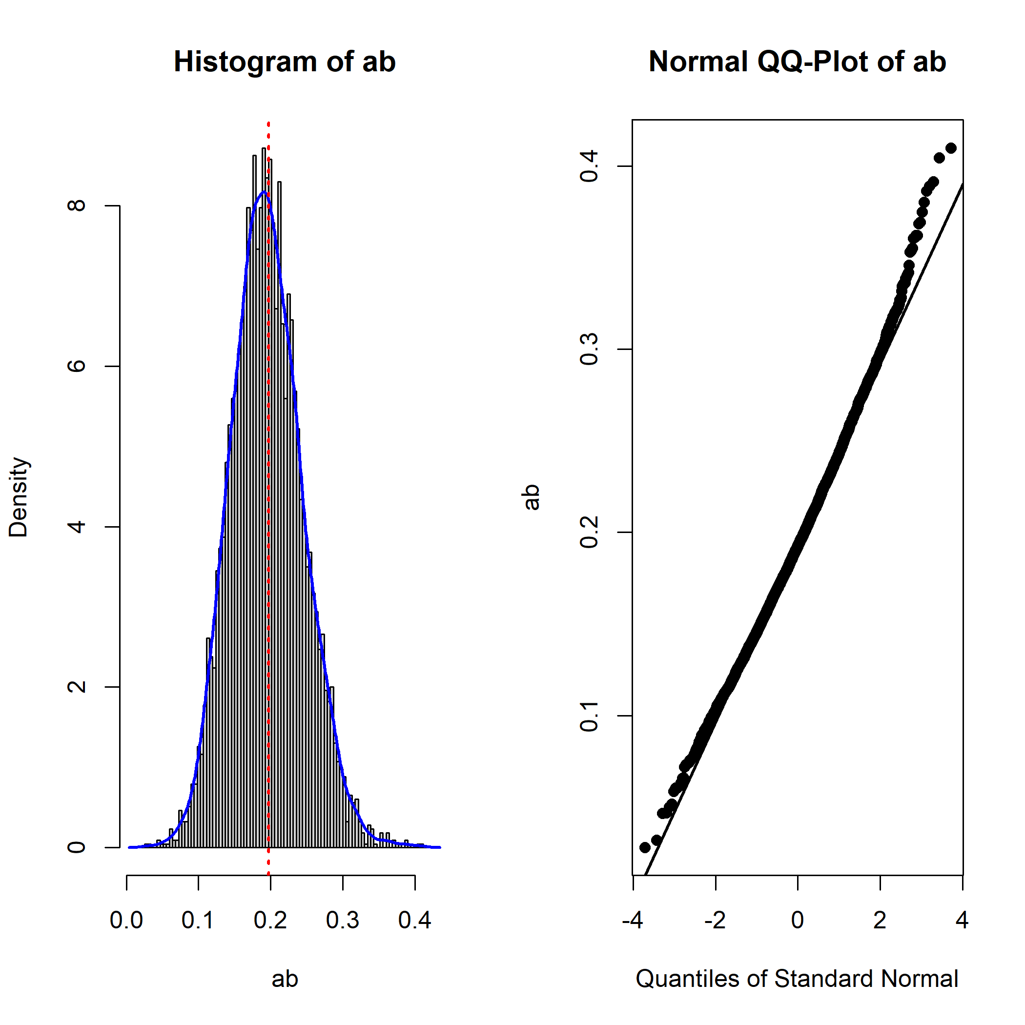

The plot suggests that, as expected, the sampling distribution of the indirect effect is not normal (positively skewed).

Standardized Solution

To plot the bootstrap estimates in the standardized solution, such as standardized regression coefficients, correlations, and standardized indirect effect, first call store_boot_est_std() to compute the bootstrap estimates in the standardized solution and store them back to the output of lavaan.²

fit <- store_boot_est_std(fit)

Once computed and stored, plot_boot() can be used again. For example, to plot the distribution of the standardized indirect effect, just set param to "ab" and set standardized to TRUE:

plot_boot(fit,
          param = "ab",
          standardized = TRUE,
          qq_dot_size = 1)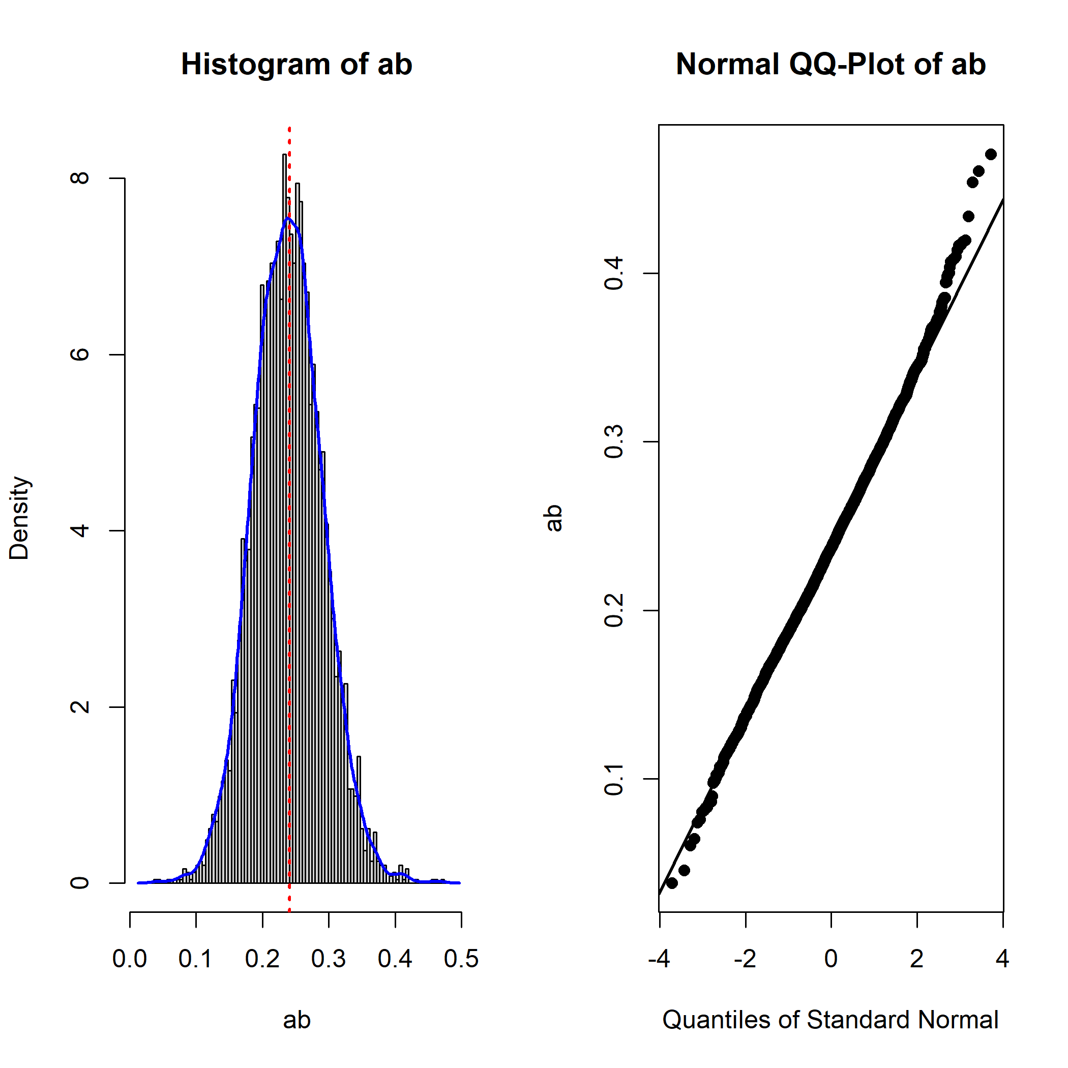

Note that it is not unusual for a parameter to have a nonnormal sampling distribution in the standardized solution. For example, this is the plot of the bootstrap estimates of the standardized path from M to Y:

plot_boot(fit,
          param = "b",
          standardized = TRUE,
          qq_dot_size = 1)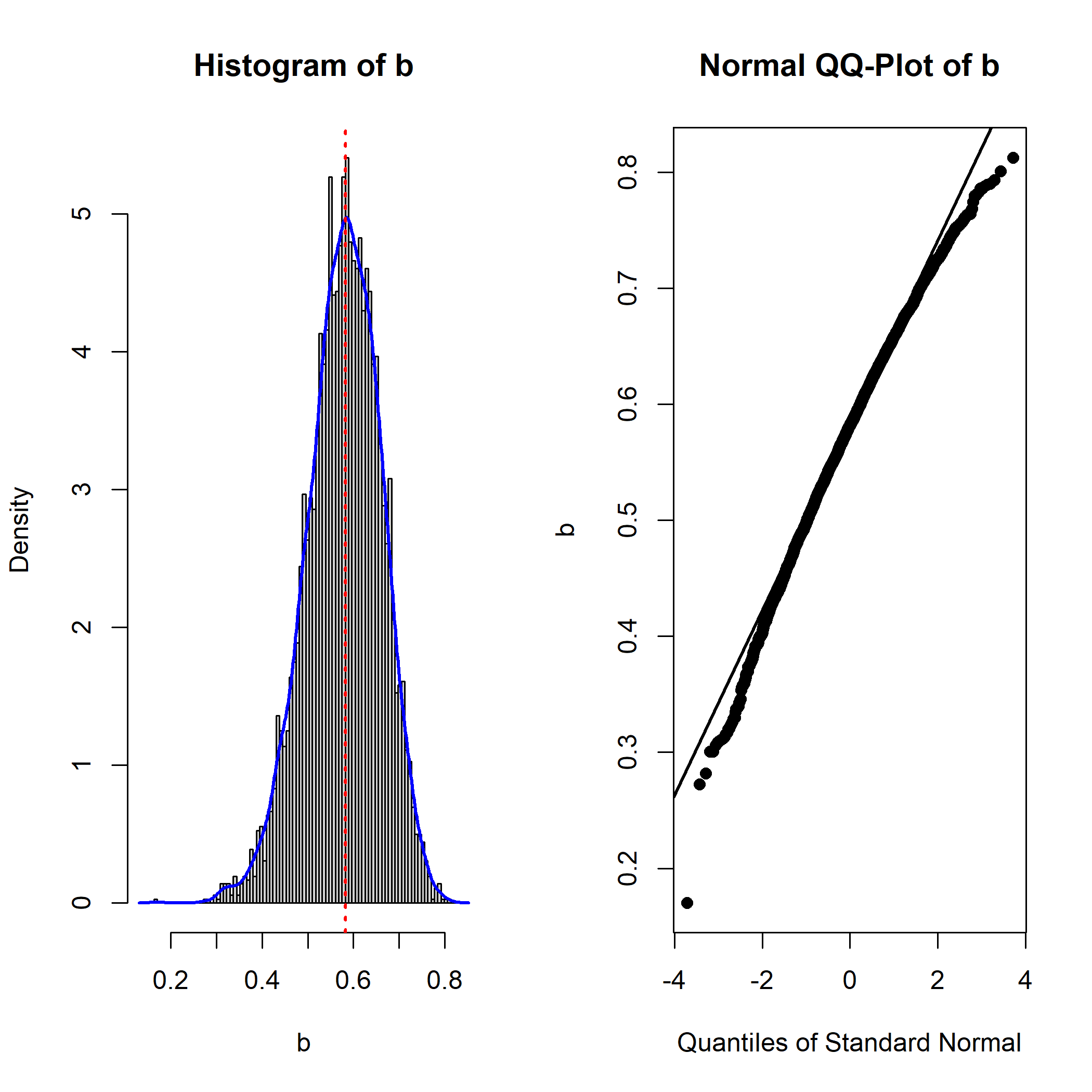

Compared to the previous plot of b in the original (unstandardized) solution, the distribution is nonnormal (negatively skewed).

Customizing the Plots

Users can customize a lot of aspects of the plot, such as the color of the lines, the number of bars, and the size of the dots in the normal QQ-plot. Please refer to the help page of plot_boot() for the arguments available.

References

Rousselet, G. A., Pernet, C. R., & Wilcox, R. R. (2021). The percentile bootstrap: A primer with step-by-step instructions in R. Advances in Methods and Practices in Psychological Science, 4(1), 1–10. https://doi.org/10.1177/2515245920911881

Shu Fai Cheung