
Workflow Demo: 4 Latent Variables
2026-09-13
demo_lav_4.RmdIntroduction
This article is part of a series of articles to demonstrate how to use semeqmodels to identify models empirically equivalent to a target model, called the original model.
NOTE: To make articles in this series self-contained, some sections are repeated across articles.
Original Model
Suppose this is the original model we fitted to the dataset
data_test_4_factor_3_item (installed with the package):
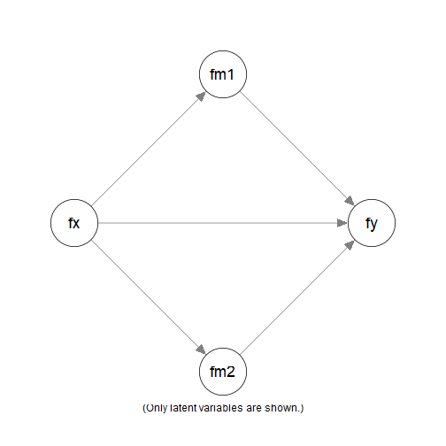
Parallel Mediation Model
This is a model:
mod <-
"
fx =~ x1 + x2 + x3
fm1 =~ m1 + m2 + m3
fm2 =~ m4 + m5 + m6
fy =~ y1 + y2 + y3
fm1 ~ fx
fm2 ~ fx
fy ~ fm1 + fm2 + fx
"
This is the lavaan results for the model:
library(lavaan)
fit <- sem(
  model = mod,
  data = data_test_4_factor_3_item
)
fit
#> lavaan 0.7-2.3166 ended normally after 43 iterations
#>
#>   Estimator                                         ML
#>   Optimization method                           NLMINB
#>   Number of model parameters                        29
#>
#>   Number of observations                           500
#>
#> Model Test User Model:
#>
#>   Test statistic                                39.488
#>   Degrees of freedom                                49
#>   P-value (Chi-square)                           0.832
#>
#>   Browne's residual (NT model-based) test
#>   Test statistic                                38.356
#>   Degrees of freedom                                49
#>   P-value (Chi-square)                           0.863
Empirical Equivalence
Suppose we would like to find some models that are empirically equivalent to this model:
In this package, two models are defined to be empirically equivalent if the following conditions are met:
They have the same model degrees of freedom.
Their absolute differences on selected fit measures are equal to or smaller than a user-defined tolerance.
See this section on a discussion of equivalence
We will start the demonstration using model , with a tolerance of 0.00001.
Generating Empirically Equivalent Models
To generate models that are empirically equivalent to a fitted model,
we can simply call eq_models() and set
original_model to the output of lavaan:
library(semeqmodels)
out <- eq_models(
  original_model = fit
)
The search can be customized if necessary. Please refer to the help
page of eq_models() for available options.
This is the text output:
out
#>
#> Number of models: 12
#>
#> The models:
#>
#>    Model
#> 1  79a7f22e
#> 2  4501984e
#> 3  ba91ae6c
#> 4  b773b38f
#> 5  ad00823e
#> 6  742796c3
#> 7  94031f00
#> 8  6d3f7956
#> 9  288c4134
#> 10 cdfe9b29
#> 11 90d21e68
#> 12 fb1b69d4
#>
#> NOTE: 'default' names are used. Call 'print()' and add 'names_to_use =
#> "long"' to use the long descriptive names, if available, for the
#> models.
The default names are generated to uniquely identify the models. Treat them as identification numbers. They are useful IDs because they are short. However, it is much easier to examine the models by drawing them.
The function eq_chisq() can be used to extract the model
s,
to verify that they have model
s
close to that of the original model:
eq_chisq(out)
#> 79a7f22e 4501984e ba91ae6c b773b38f ad00823e 742796c3 94031f00 6d3f7956
#> 39.48751 39.48751 39.48751 39.48751 39.48751 39.48751 39.48751 39.48751
#> 288c4134 cdfe9b29 90d21e68 fb1b69d4
#> 39.48751 39.48751 39.48751 39.48751
fitMeasures(fit, "chisq")
#>  chisq
#> 39.488
These models also have model degrees of freedom equal to that of the original model:
eq_df(out)
#> 79a7f22e 4501984e ba91ae6c b773b38f ad00823e 742796c3 94031f00 6d3f7956
#>       49       49       49       49       49       49       49       49
#> 288c4134 cdfe9b29 90d21e68 fb1b69d4
#>       49       49       49       49
Drawing the Models
To draw the models, the function partables_plots() can
be used. It uses the function semPlot::semPaths() from the
semPlot package to draw the model. Therefore, basic
knowledge of semPlot::semPaths() is required.
To draw the model, we need a common layout in the form of a matrix of names:
# Set the layout of the plots
m <- matrix(
  c(  NA, "fm1",   NA,
    "fx",   NA, "fy",
      NA, "fm2",   NA),
  nrow = 3,
  ncol = 3,
  byrow = TRUE)
m
#>      [,1] [,2]  [,3]
#> [1,] NA   "fm1" NA
#> [2,] "fx" NA    "fy"
#> [3,] NA   "fm2" NA
We can then generate the plots:
p <- partables_plots(
  out,
  original_model = fit,
  structural = TRUE,
  layout = m,
  label.cex = 1.2,
  sizeLat = 11,
  edge.width = 5,
  asize = 5,
  curve_cov_settings = list(base_curve = 4)
)
The argument curve_cov_settings, with
list(base_curve = 4), is used to make the curves for
covariances easier to read.
We can then call plot() to plot the models. By default,
they will be drawn one by one. To draw them in a grid, use the arguments
ncol and nrow:
plot(
  p,
  ncol = 4,
  nrow = 3,
  title_adj = 2
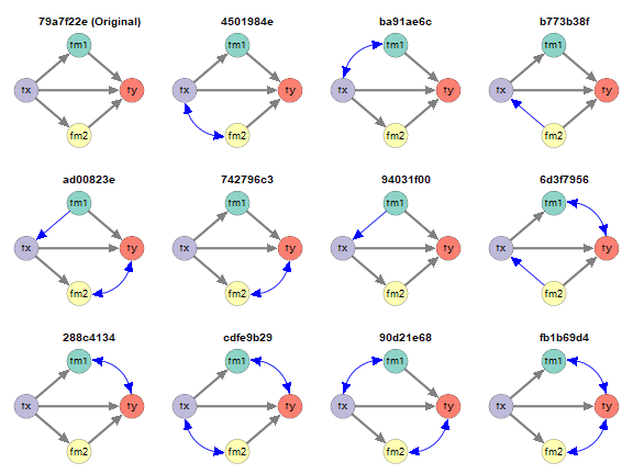
)
Empirically Equivalent Models
The model labeled Original is the original model. The
other models are empirically equivalent to this model in this
dataset.
By default:
Paths or covariances different from the original model are colored.
Covariances are displayed using curves.
There are other ways to customize how the models are drawn. Please
refer to the help page for plot.partables_plots().
Filter the Models
The package semeqmodels has functions for selecting
models, listed here.
They can also be used to filter the output of
partables_plot(). Some of them are demonstrated below.
fx Must Not Be a DV (y-variables)
Suppose that we have reasons to argue that fx cannot be
an outcome of any other variables in the model. For example,
fx is measured one month before the other variables.
We can use must_not_be_y() to specify variables that
cannot be a “DV.”
p1 <- p |>
  must_not_be_y(
    vars = "fx"
  )
plot(
  p1,
  ncol = 4,
  nrow = 2,
  title_adj = 2
)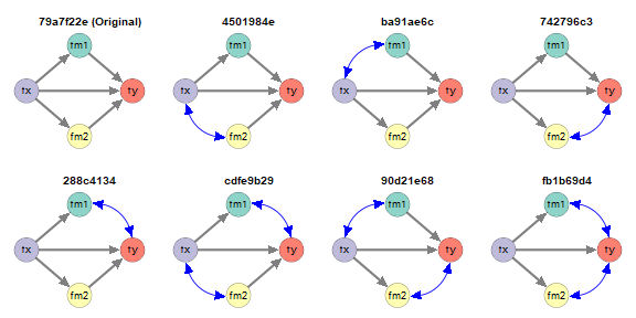
fx Must Not Be a y-Variable
Note: A variable is a “DV” if it appears as the outcome of at least one other variable. Therefore, a mediator is also a DV.
Must Have Some Direct Paths
Suppose that we have theoretical reasons to argue that
fm1 and fm2 must be affected directly by
fx, and so would like to keep models with these two
paths.
We can use have_pars_all() to specify paths that must be
present in a model
p2 <- p |>
  have_pars_all(
    pars = c("fm1 ~ fx",
             "fm2 ~ fx")
  )
plot(
  p2,
  ncol = 4,
  nrow = 1,
  title_adj = 2
)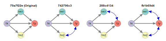
Some Paths Must Be Present
Must Not Have Any Paths from fm1 to
fm2
Suppose that, theoretically, fm1 cannot have any effect
on fm2, directly or indirectly. We can use
must_not_have_paths().
p3 <- p |>
  must_not_have_paths(
    y_on_x = "fm2 ~ fm1"
  )
plot(
  p3,
  ncol = 4,
  nrow = 3,
  title_adj = 2
)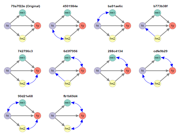
No Paths from fm1 to fm2
Chaining the Selections
The selectors can be chained together using |>.
p5 <- p |>
  must_not_be_y(
    vars = "fx"
  ) |>
  have_pars_all(
    pars = c("fm1 ~ fx",
             "fm2 ~ fx")
  ) |>
  must_not_have_paths(
    y_on_x = "fm2 ~ fm1"
  )
plot(
  p5,
  ncol = 4,
  nrow = 1,
  title_adj = 2
)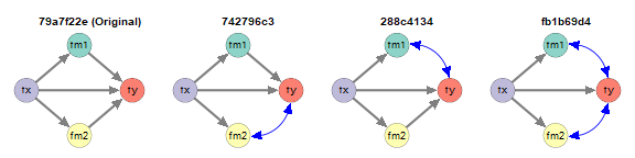
Chained Filter
Final Remarks
Customize the Search
There are many other ways to customize the search and the plots. Please refer to the corresponding help pages for details.
Demonstrations of other models and cases can be found in the other demonstration articles
Equivalence-In-Principle and Empirical Equivalence
The concept of mathematical equivalence models, or two models being equivalent in principle (Lee & Hershberger, 1990), has a long history in the literature on structural equation modeling Williams (2012). Two models are considered to be mathematically equivalent if they necessarily imply the same covariance matrix regardless of the data. There are methods to generate them and tools to generate them automatically (e.g., Lee & Hershberger, 1990).
Our definition of empirical equivalence is similar to empirical occurrence of equivalence (EOE, Lee & Hershberger, 1990). However, we include the requirement of equal degrees of freedom: two models must also be equal in parsimony. We also allow for the possibility of using any fit measures deemed appropriate (e.g., CFI, RMSEA), and also the use of tolerance values that are appropriate for a situation.
Although our focus is on empirical equivalence, two models that are mathematically equivalent in the conventional sense are necessarily empirically equivalent. Note that the reverse is not true: two models that are empirically equivalent are not necessarily mathematically equivalent.
Nevertheless, when the tolerance is set to be very small, the models identified, though not necessarily, are likely to be mathematically equivalent. Therefore, the package can also be used to identify models that are likely mathematically equivalent.